Examples
Choose a chart to open its live preview and source. Examples mount individually.
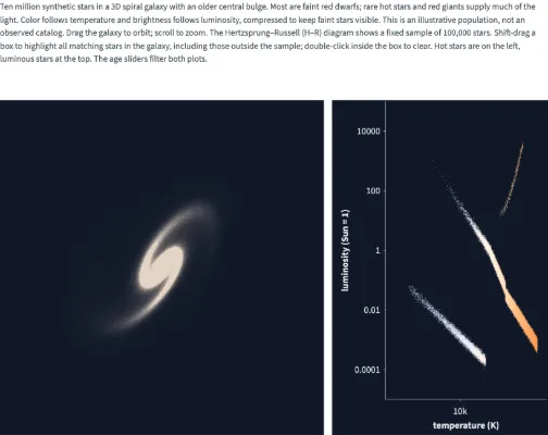
Ten million stars, filtered live
Ten million synthetic stars generated by Data(rows) on the GPU, age-filtered live, with a fixed 100,000-star H–R sample that brushes the whole galaxy. Square points and additive starlight.
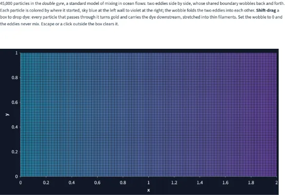
Mixing in a double gyre
45,000 particles ride the double gyre, a standard model of mixing in ocean flows, stepped on the GPU by Simulate at the display's rate. Each is colored by where it started, and the wobble of the eddies' boundary folds the two into each other; a Shift-drag box drops dye that the particles carry downstream in thin filaments (the brush feeds the simulation's state). A slider sets the wobble: at 0 the eddies never mix.
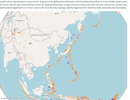
A globe with streamed map tiles
An orthographic globe whose basemap streams in as you turn and zoom it: OpenStreetMap vector tiles from VersaTiles, loaded at the zoom the view needs, from the whole planet down to a city's streets, with their credit in the corner. Every magnitude 4.5+ earthquake of 2024 (USGS) sits on top, sized by magnitude and colored by depth.
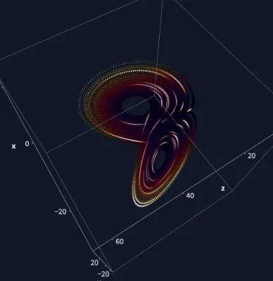
Lorenz attractor
Sixty thousand Runge-Kutta steps of the Lorenz system trace its butterfly; on the GPU every point then moves on at the Rayleigh number you drag, collapsing onto two fixed points below about 24.7. A glowing 3D orbit with sparks that run along it in time order (evaluated on the GPU from @time), linked to the butterfly projection: brush a region and the 3D view keeps only those points lit while a speed histogram counts them.
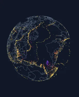
Earthquakes beneath the globe
Every earthquake of magnitude 4.5+ in 2024 (6,397 events, USGS) placed at its true depth inside a see-through globe, where deep quakes trace subducting slabs; a slider exaggerates the depths. Brush a region on the map and a period on the timeline; the brushes combine, the globe keeps the matching quakes lit, and a log-scale histogram shows the Gutenberg–Richter law.
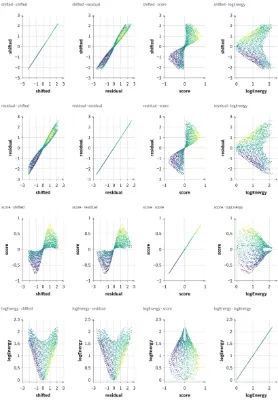
Calculated scatterplot matrix
Sixteen coordinated views of four calculated fields. Hover, select, and Shift-drag to brush across cells. Counts are per cell; 25,000 rows produces 400,000 plotted instances.
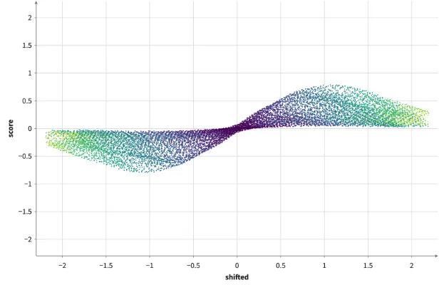
Large calculated point cloud
Three sequential Calculate scopes share intermediate columns. Change gain to update the final stage; hover, select, and Shift-drag to brush the resulting point cloud. No sampling limit is applied.
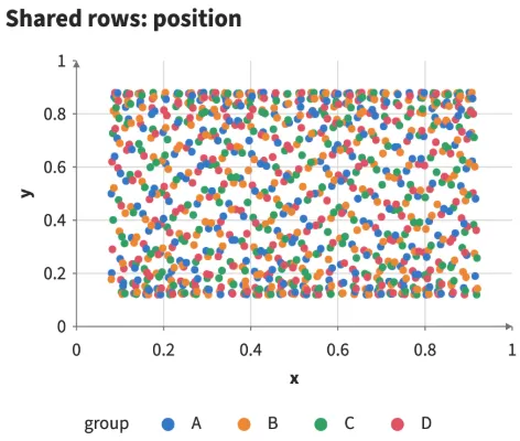
Coordinated interaction dashboard
Hover either shared view: the same row enlarges in both. Click/Shift-click selects/toggles; Shift-drag brushes. Drag the brush or click away to clear it. The filtered view updates while brushing. The independent table must not react, even though its IDs and values match.
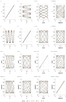
Interaction matrix and scrolling
The same observation appears in all 16 cells. Hover should enlarge it everywhere; selection and brushing should coordinate by row, not category. Scroll away and back, then repeat. Compare cache sizes 0 and 64. Pan and zoom are independent in this example.
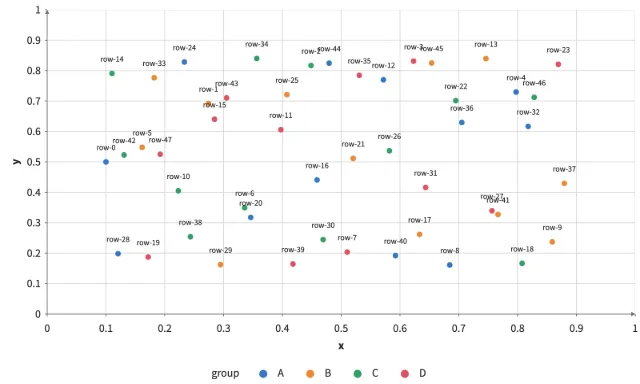
Keyed updates under interaction
Select a few points, hover, then step the frame or reverse the rows. Surviving IDs retain selection; removed IDs disappear. Point fades last 500 ms and label fades last 200 ms. No automatic timer runs: every update is explicit. Hover size is immediate unless the configured animation applies.
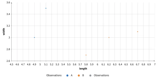
Data shortcuts
Composable data scopes, coordinate frames, and shared navigation.
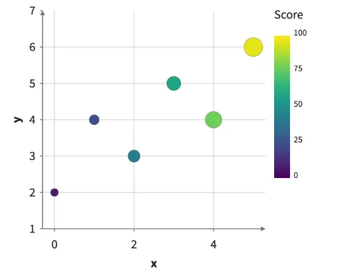
Shared and independent scales
Share one normalization across color and size, isolate same-named columns in separate tables, and map ordered categories.
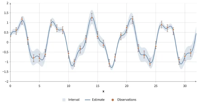
Signal and uncertainty
Animated intervals, estimates, observations, error bars, legends, and an independent overview.
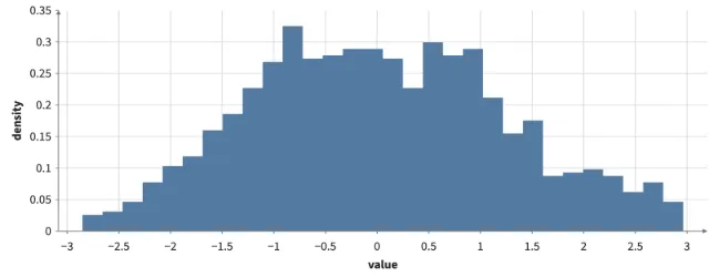
Histogram bins
A Slider input sets a Histogram's bin count.
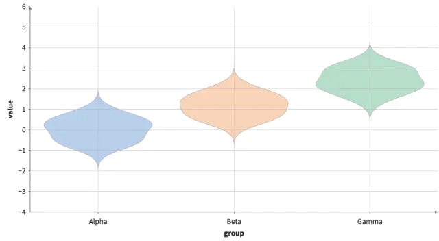
Violin plot
Grouped GPU density bands with categorical color.
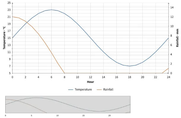
Twin coordinate frames
Composable data scopes, coordinate frames, and shared navigation.
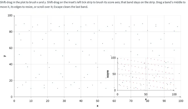
Brushing frame strips
Shift-drag on an inset frame's tick strip to brush its own axis. The band stays on the strip; a column shared with other strips shows on each of them.
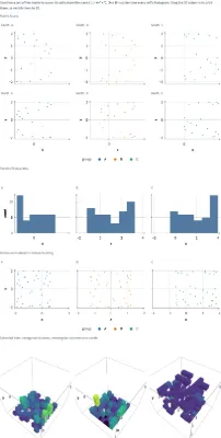
Facets & transforms
Derived data scopes, repeated plots, and extruded bins.
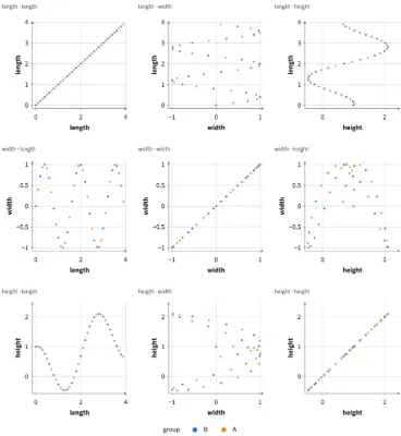
Scatterplot matrix
Facet pairs: lazy pair views, one domain per field on x and y, and consistent category colors.
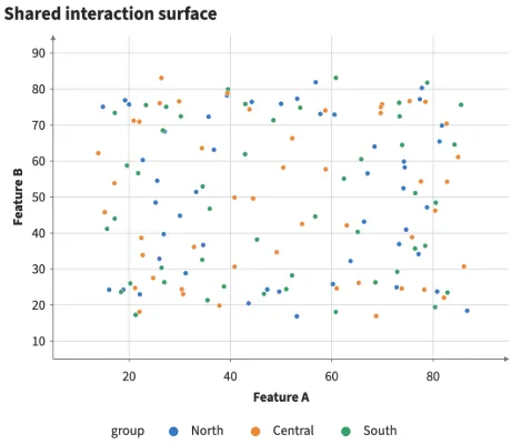
Coordinated interaction explorer
Coordinate hover, click selection, a movable brush, and filtered projections across three views.
Keyed enter and exit
Keep matching observations continuous while new keys enter and removed keys exit.
Force layout · 2D
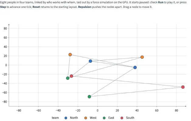
A small team graph laid out by a force simulation on the GPU: run, step, reset, repulsion and dragging.
Long time series
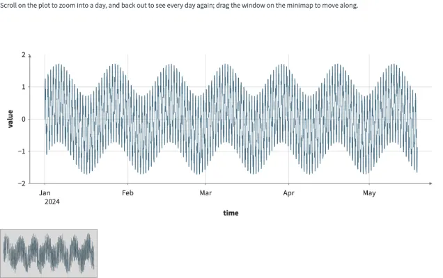
Zoom into a long signal with adaptive peak-preserving detail or draw every point.
Polar radius
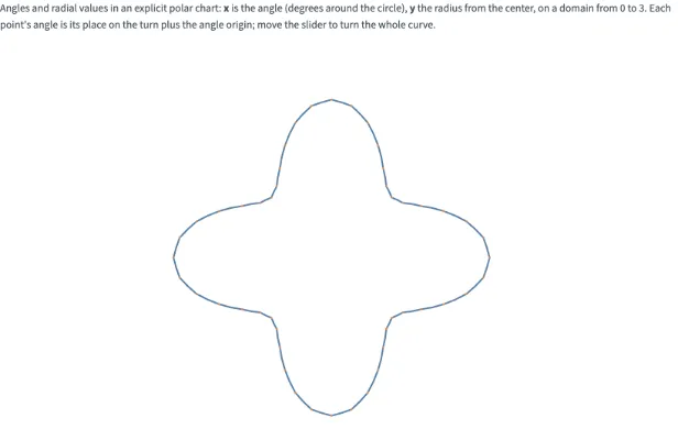
Angles and radial values in an explicit polar chart.
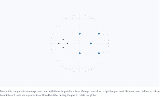
Polar and tangent insets
A warped chart and a rigid tangent inset on a rotatable orthographic sphere, with a 24-unit polar dial.
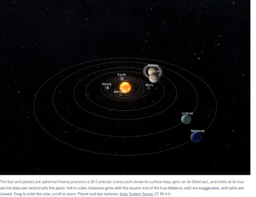
Solar system
The Sun and the eight planets as textured spherical Frames placed in a 3D scene. Each planet orbits at its true period, spins on its tilted axis, and is lit by the Sun; Saturn's rings are an Image in a polar Frame turned onto its equator.
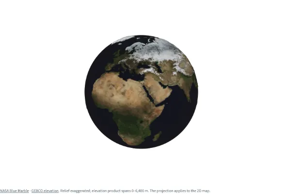
Earth relief
NASA imagery over an elevation surface, with adjustable relief and directional lighting.
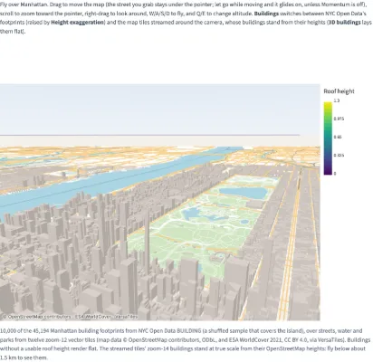
Manhattan building flyover
Fly over 10,000 of Manhattan's 45,194 building footprints, over streets, water and parks from vector tiles, or stream the map tiles around the camera with their own buildings standing.
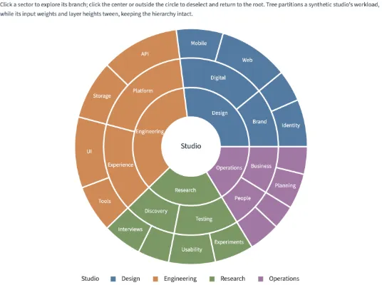
Zoomable sunburst
Click to explore a weighted Tree partition with input weights and layer heights tweened before layout. The Svelte and Python scenes work in standalone HTML.
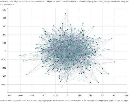
Large force graph
Explore seeded graphs of 64 to 10,000 nodes, thin edges, dragging, and a linked overview in 2D or 3D.
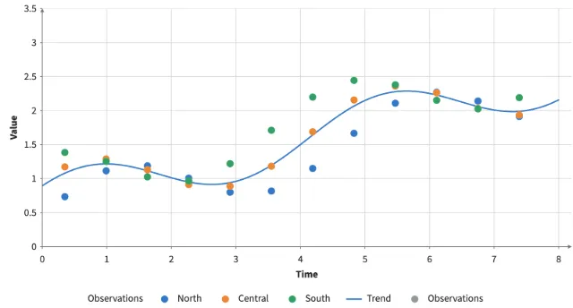
Theme presets
Compare every built-in theme on the same plot, including backgrounds, axes, marks, categorical colors, and its legend.
Additional examples
Marks
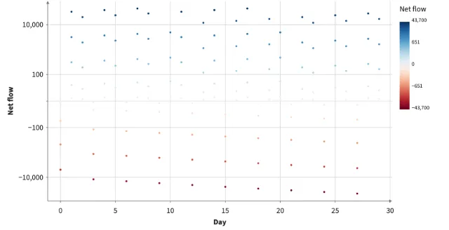
Symlog axis and a diverging scale
Values that cross zero with a wide range: a symlog y axis is linear within ±10 and logarithmic beyond, so small days and large ones both read, and outflows are drawn (a log axis would drop them). The color scale's midpoint puts RdBu's white at 0 and uses both ends of the colormap.
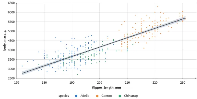
A fitted curve that refits under a brush
Smooth fits a curve (linear, polynomial, log, exp or power) with its 95% confidence band on the GPU: penguins' body mass against flipper length. Brush some penguins and the fit follows them.
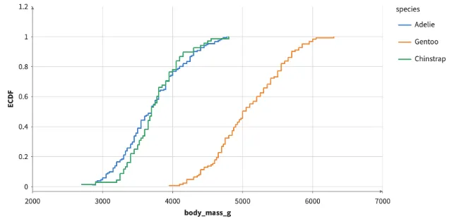
ECDFs by species
Each penguin species' body mass as steps: the fraction of its penguins at or below each mass.
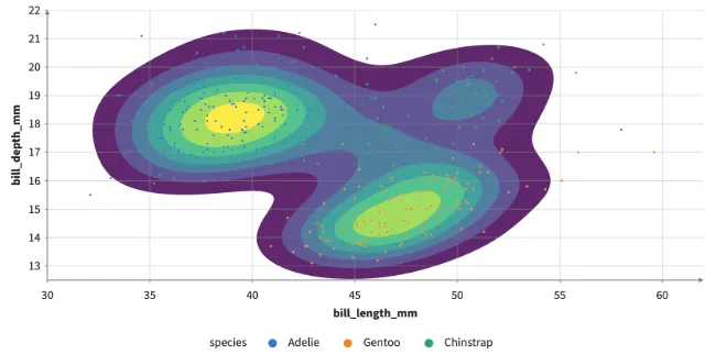
Density contours
The density of penguins' bill length against depth as filled bands, contour lines or both, on the GPU: Density, then Contour's marching squares.
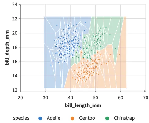
Voronoi cells, hulls and a Delaunay triangulation
Each penguin's Voronoi cell (hover one to highlight its penguin), each species' convex hull, and the Delaunay triangulation, drawn by Polygon and Segments.
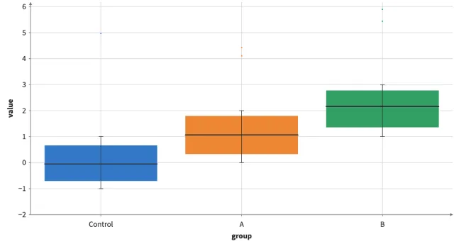
Box plot
Quartiles, Tukey whiskers, medians, and source-linked outliers.
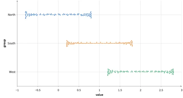
Swarm plot
Deterministic glyph-aware dodge with stable observation identities.
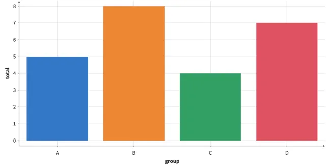
Bar chart
Categorical bars composed from derived geometry and instanced prisms.
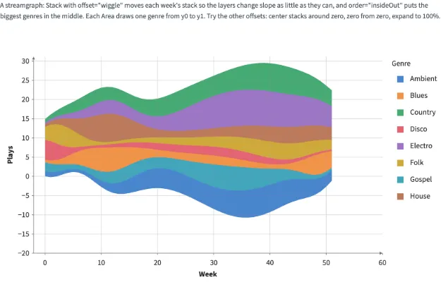
Streamgraph
Stack with offset="wiggle" and order="insideOut": each week's stack moves so the layers change slope as little as they can, the biggest genres in the middle, and an Area per genre draws it. The controls switch the offset and the order. Area transitions animate by default; the Animate control can turn them off.
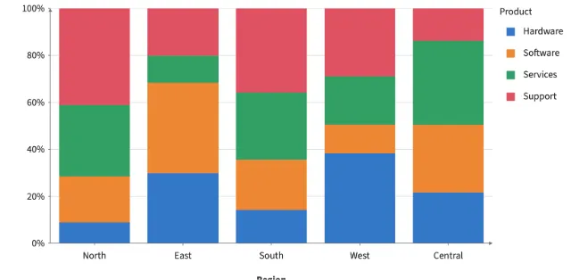
100% stacked bars
Stack with offset="expand" scales each region's stack to span 0 to 1, so each Bar segment is a product's share of the region's sales.
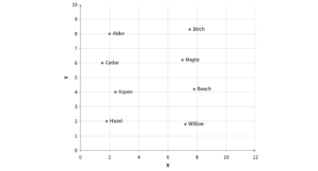
Point labels
Named observations with GPU-rendered labels that follow pan and zoom.
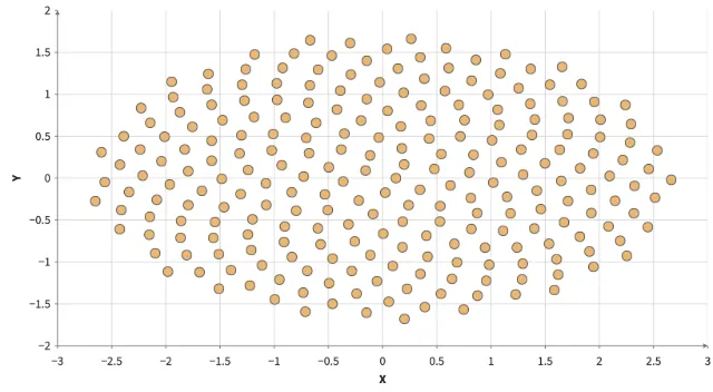
Point symbols
Eight flat symbols, inward outlines, rotation, and GPU picking.
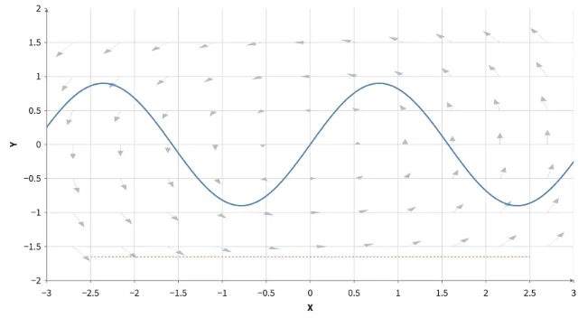
Lines & vector fields
Connected lines, independent segments, dashes, and endpoint arrows.
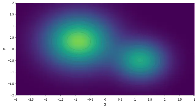
Density & surfaces
One GPU heatmap, fixed color bounds, contours, and an optional 3D surface.
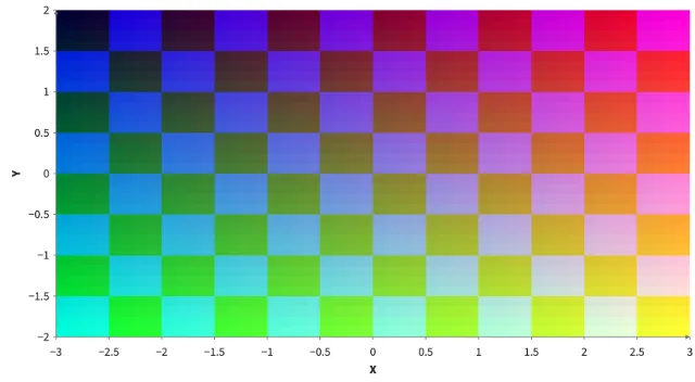
Images
Grayscale and RGB tensors retain their original colors, with nearest-neighbor pixels.
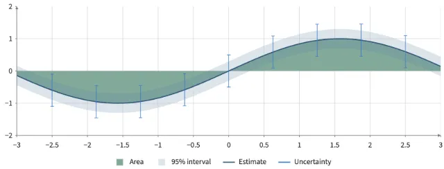
Legends & uncertainty
Series legends, GPU colorbars, filled areas, and capped uncertainty intervals.
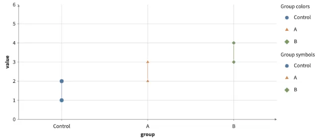
Named data & categories
Named columns, shared categorical colors and symbols, categorical axes, and GPU dictionary columns.
Composition
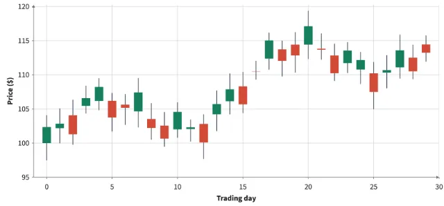
Portable candlestick template
OHLC candles composed from ErrorBars, Calculate, Filter and Rect. Download the template and supply your own price table.
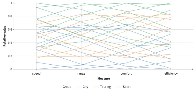
Portable parallel coordinates
Fold and Normalize turn a wide table into comparable dimensions. A portable Line template draws one profile per observation.
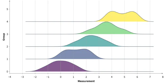
Portable ridgeline template
Grouped Gaussian densities in one shared frame, packaged as a downloadable template. Change the data, bandwidth and ridge height.
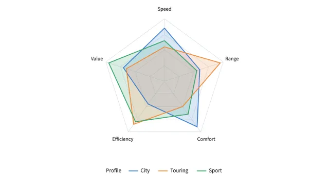
Portable radar template
A portable polygon template maps normalized scores to a radar chart. Rings, spokes and labels are supplied by the host.
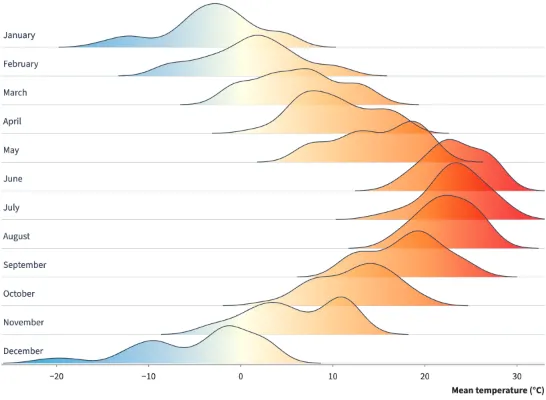
Ridgeline temperatures
Twelve monthly temperature densities from Lincoln's 2016 weather, with overlapping ridges and a shared blue-to-red temperature gradient.
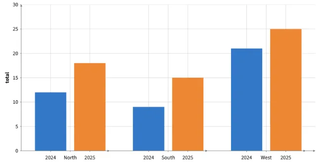
Embedded facets
Facets inside a Plot partition its frame and share its renderer and camera. For grouped bars, use Bar with arrange="group".
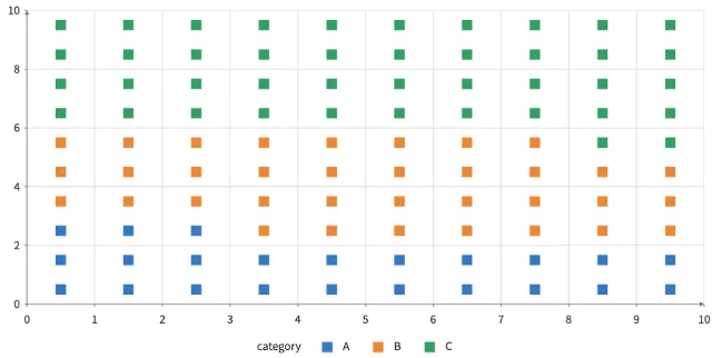
Waffle grid
Integer counts expand into source-identified unit squares, ordered left to right and bottom to top.
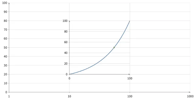
Nested scales
A child interval maps through its parent’s logarithmic scale.
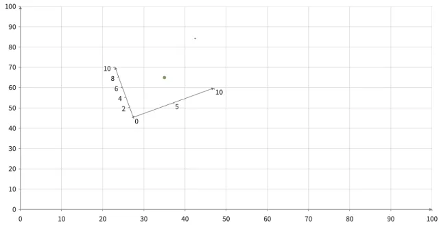
Anchored frame
Pan and zoom: the child frame stays 160 by 100 CSS pixels, anchored at its parent data position.
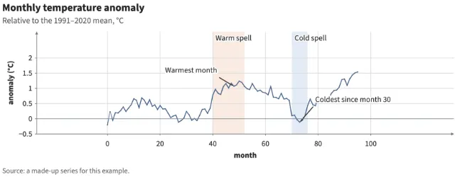
Titles, bands and callouts
A plot's title, subtitle and caption are part of the plot and its exports; bands shade a span of an axis behind the marks and grid; callouts point at a value with a note.
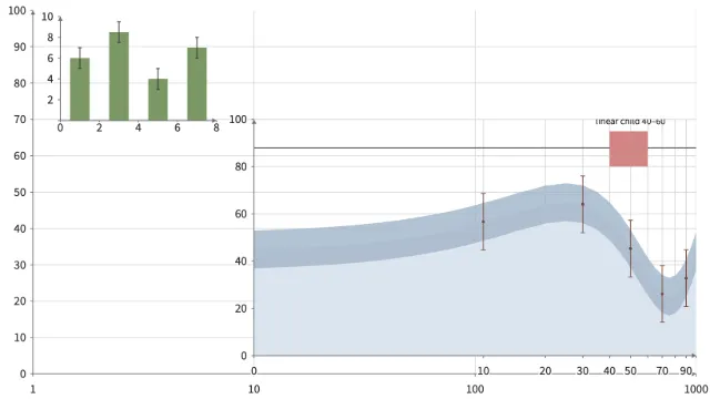
Marks in nested frames
Area, ErrorBars, Rect, and curved Segments inside a linear child of a log parent, and bars with error bars in an anchored inset that keeps its pixel size while you pan and zoom.
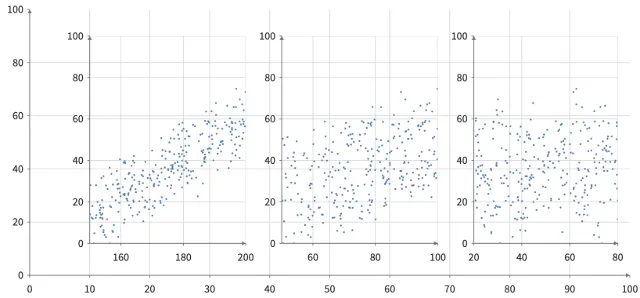
One brush, three strips
Three child frames plot score against different fields. Shift-drag any tick strip: the shared score brush appears on every strip. Drag band ends to resize, the middle to move, scroll to scale, and use arrow keys or Escape.
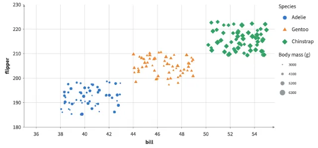
Legend channels
Colored symbols when one column drives fill and shape, a size ramp for a numeric column, and one legend for a facet grid that hides a species in every cell.
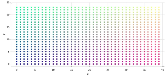
RGB colors from data
Color each point from red, green, and blue columns. Integer data is 0-255 and float data 0-1; RGB colors bypass scales and legends.
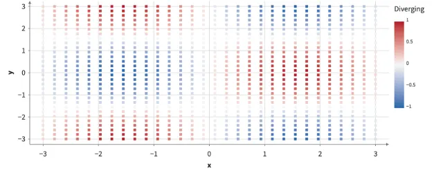
Custom colormaps
A diverging colormap from three colors and a positioned ramp that saves its strongest colors for the top of the domain. Legends and exports follow.
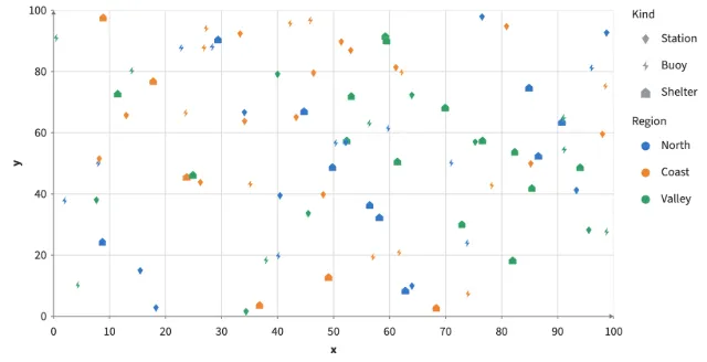
Custom point shapes
Register polygons as point shapes and map a column to them with shape and shapeScale; the legend and SVG export draw the same polygons.
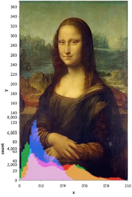
Mona Lisa histogram
Every pixel of the painting is a data-space square with RGB fill, and an RGB histogram sits over its lower part, its three channels screen-blended so overlaps add up to white as in the D3 notebook. Brush a region and the histogram counts only those pixels. After the D3 notebook of the same name.
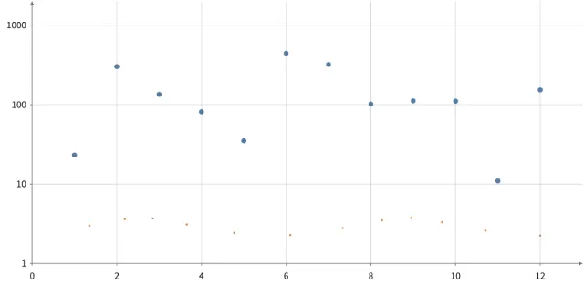
animate, enter/exit, and @time
animate() moves one channel per row in its scale space (geometric on this log axis) with enter and exit values for rows that come and go, while @time satellites on fixed rows of their own orbit continuously without blocking settlement.
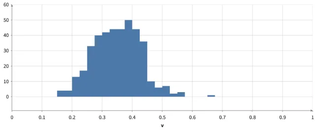
tween and @time in the pipeline
A tweened column moves as data: the histogram under it re-bins its rows every frame while they glide to new values, and a Filter on @time lets points in as the view clock passes them.
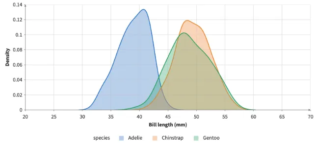
One density per group, one frame
Partition repeats its children once per group inside a single frame, sharing the parent's scales, axes, and legend. Here a Density transform runs per species so the curves overlay; Facet would give each species its own cell instead.
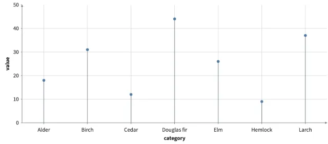
Lollipop chart
A stem from the baseline to each value, on either side of it, with a point at the end. Lollipop is a built-in template: BarGeometry places each stem, Segments draws the stems and Points the heads.
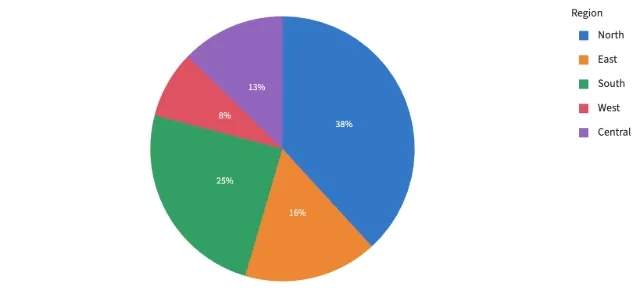
Pie chart
Each region's share of the sales, clockwise from 12 o'clock, labeled with its percentage. Pie is a built-in template: a PieGeometry transform and Rects in a polar Frame, which it places in a Cartesian Plot.
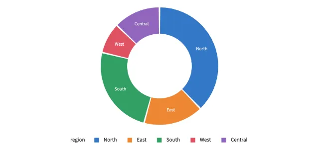
Donut chart
innerRadius opens the hole and padAngle separates the sectors. Keyed rows tween each sector's angles when the values change.
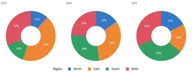
Pies in a Facet
Small multiples: a Facet repeats the Plot once per year, and each Pie sums its own year's sales, with one legend for the row.
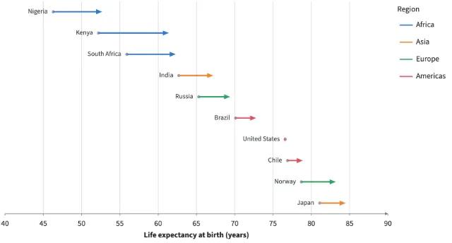
Before and after arrows
connect() pairs two marks' rows by key and draws one arrow per pair. The 2000 values are points, the 2021 values an invisible Anchor, and the arrows take their color from the shared table.
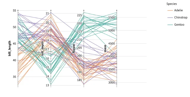
Parallel coordinates from connections
An embedded Facet with fields makes one cell per measurement, in which value is that measurement, each with its own y scale titled by the measurement, and a Frame in every cell sets x from 0 to 1, so the points sit on each cell's axis. One Line connects the points across the cells in facet order, and every cell shows the same penguins, so rows match without a key. Shift-drag on any axis to brush that measurement; brushes on several axes combine.
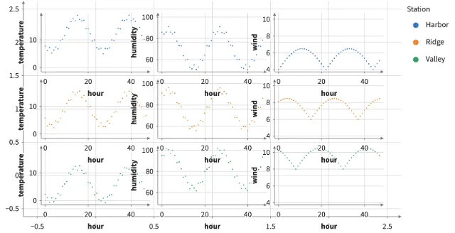
One cell per variable
Facet fields repeats its children once per field over the same rows; inside each cell, value is that field. Each field keeps its own y scale while columns of the table stay shared. With row="station" the fields form a grid by station, a field keeping one scale down its column.
Combinations
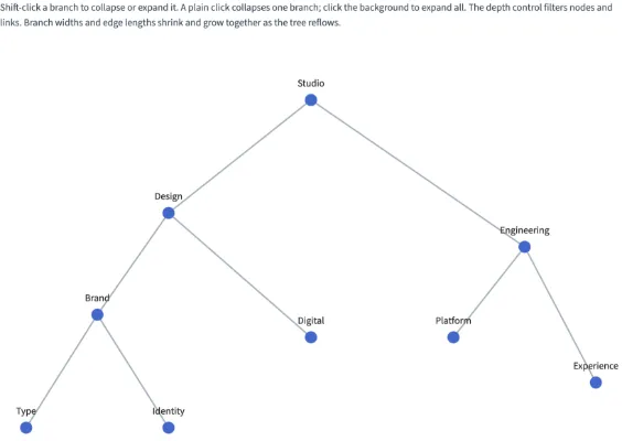
Expandable tree
Collapse branches and filter by depth while GPU subtree widths and unequal edge lengths animate. Paired Svelte and Python scenes.
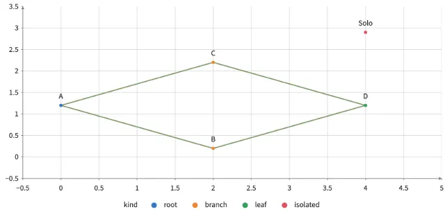
Positioned graph
Node positions computed from node columns, with edges gathered from those positions.
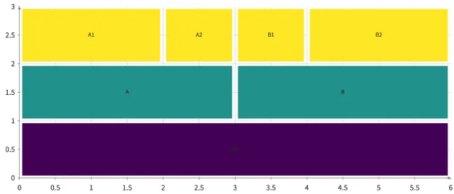
Tree icicle
Nested hierarchy rectangles from Tree partition bounds.
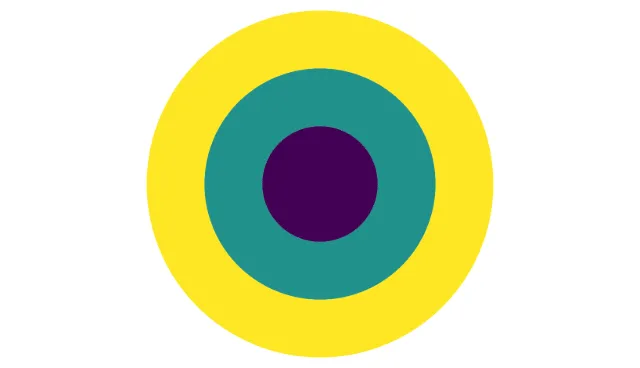
Tree sunburst
Tree partition spans mapped to annular sectors.
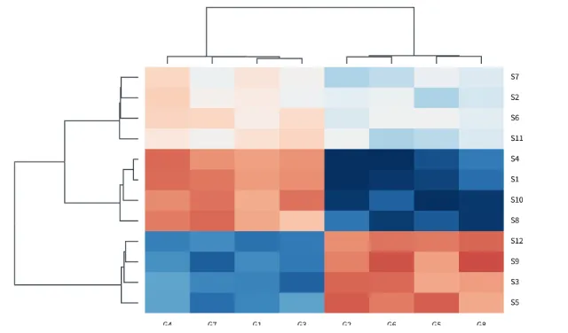
Clustered heatmap
A heatmap sorted by two dendrograms, as seaborn's clustermap: Tree mode="cluster" draws each precomputed linkage to scale by its merge heights, in Frames that share the heatmap's rows and columns, and labels the leaves by their order.
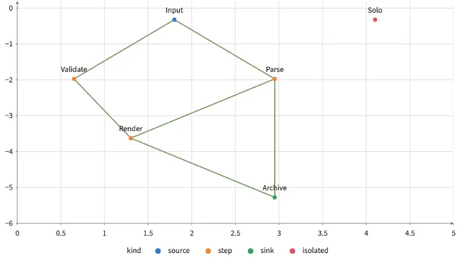
Layered DAG
Sugiyama layout with routed links and node sizes.
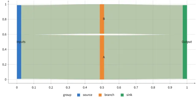
Sankey flow
Acyclic weighted network with bands attached to node intervals.
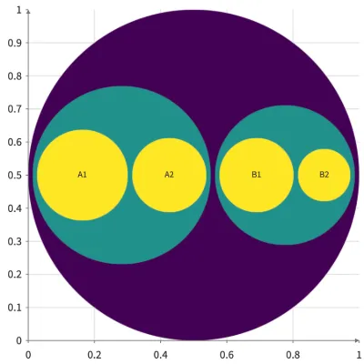
Circle packing
D3 circle packing sized by leaf values, with centers and radii on Nodes.
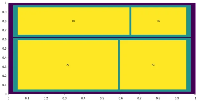
Treemap
D3 treemap bounds from a weighted hierarchy.
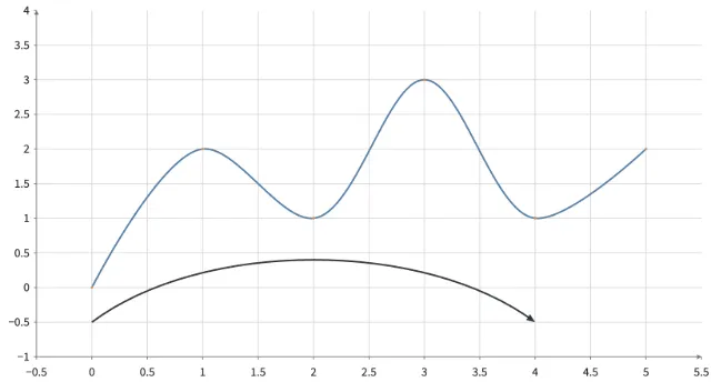
Curved paths
GPU curves and camera-facing arrowheads with bounded subdivision.
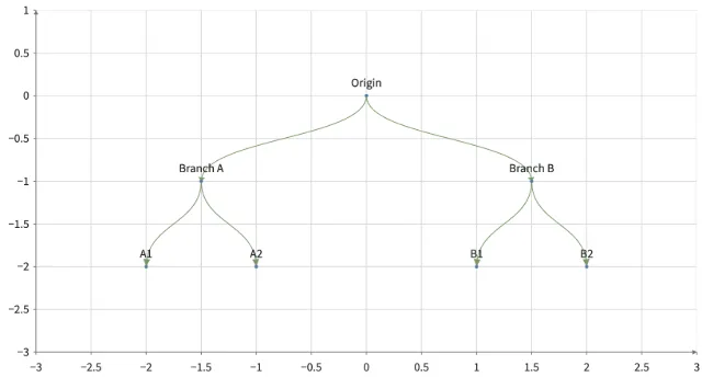
Rooted tree
A deterministic spanning tree with labels and curved directional links.
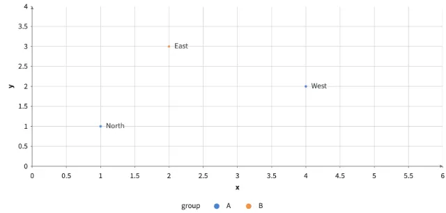
Shared mappings
One mapping scope drives positions and styles for points and labels.
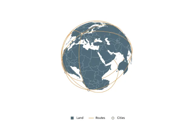
Globe and routes
Regions, great-circle paths, outlined cities, projection switching, legends, and navigation.
Interaction
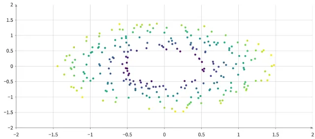
Particles without an uploaded table
Data(rows) generates row indices, ones and fixed random values on the GPU; Simulate moves the particles without a dummy table from Python.
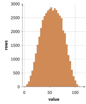
Brushed filter chain
Shift-drag to brush 50,000 points; a histogram (Filter > Bin) and per-level means (Filter > Group) follow the brush. A Filter keeps its input's rows and marks the kept ones, so a moving brush changes no array length and compiles no new GPU kernels.
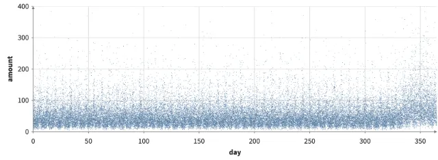
Running totals under a brush
Shift-drag to brush 50,000 transactions; the brushed rows are sorted by day, then a running sum and a 500-row moving average follow the brush (Filter > Sort > Window > Line).
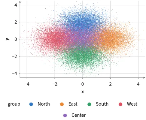
Brushed distributions
Shift-drag to brush 60,000 points in five clusters; violins and box plots of each group's values are recomputed from the brushed rows on every move, with no GPU kernels compiled while dragging.
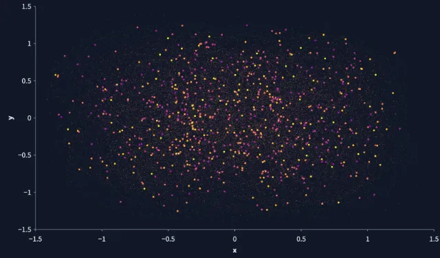
Moving particles
1,500 particles circle at their own speeds: Slice interpolates every particle's position at the current time on every animation frame, and a slider filters them by speed. Neither playing nor filtering compiles new GPU kernels once warm.
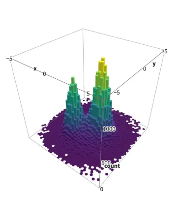
Half a million points, one slider
A slider filters 500,000 points by magnitude into a 3D hexbin and a histogram. A Filter that keeps under a quarter of a large input packs the kept rows into a few fixed lengths, so the work after it follows the selection and each length compiles once.
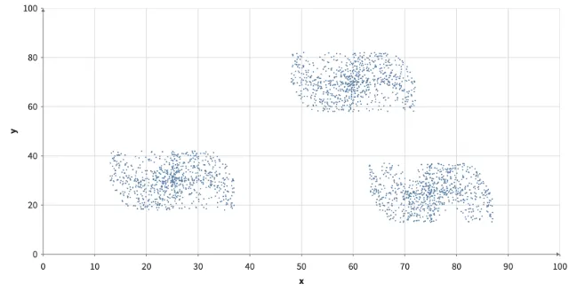
Nearby points
Move the pointer over the clusters: every row within the radius grows, including all overplotted rows at a cluster center, and the rest shrink. Adjust the radius with the slider.
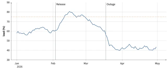
Crosshair and rules
Move the pointer over a time series: the crosshair follows it with a readout of each value. A dashed rule marks a threshold and gray rules mark events from a second table, labeled at the top of the frame.
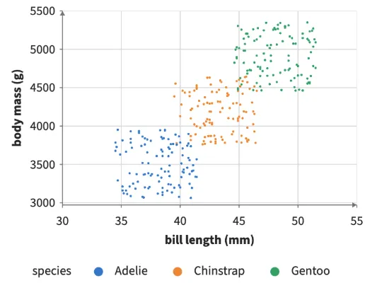
Tooltips
Point near a penguin: the tooltip shows the nearest one within 16 pixels, with chosen fields, labels and formats, and @tooltip enlarges it; a histogram's bars show their bin and count.
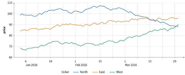
Unified x tooltip
Move the pointer along the dates: one tooltip lists every series' value at that date, with a marker on each line, beside a Crosshair's vertical rule.
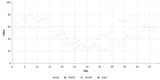
Nearby along x
Single-axis nearby in data units picks every series at the day under the pointer, whatever the pointer's height, and labels them.
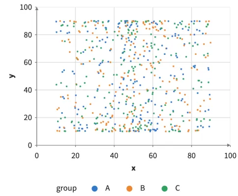
Respond only while active
@any_brushed and @any_selected are 1 on every row while anything is brushed or selected, so the other rows shrink only then. Shift-drag or click in either plot; clear to restore every row.
Joining two tables
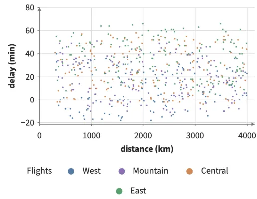
Flights name their origin airport by code; Join adds each airport's region from a second table, so the flights are colored, grouped on an axis and brushed by it.
Dragging points
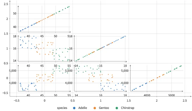
Drag a point in a scatterplot matrix: the drag writes offsets on the table's rows, and every cell that reads moved() of the dragged column follows.
Dragging cities on a map
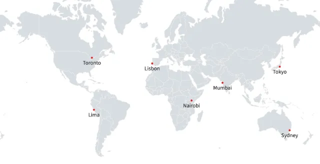
Drag a city on a Mercator map: the drag goes back through the projection and writes offsets in degrees; the point and its label both read moved().
Data selections and brushing
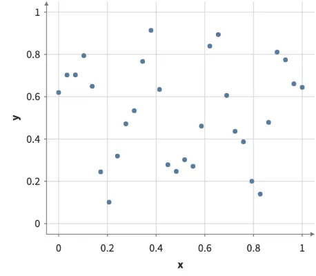
Click or brush observations and filter another plot through data-owned virtual fields.
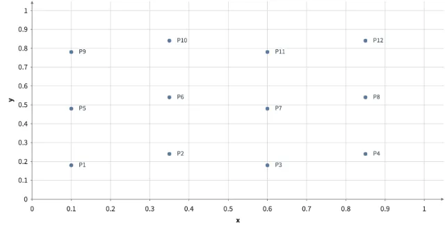
Hover and click selection
Highlight hovered rows, toggle keyed selections, and update selection state from code.
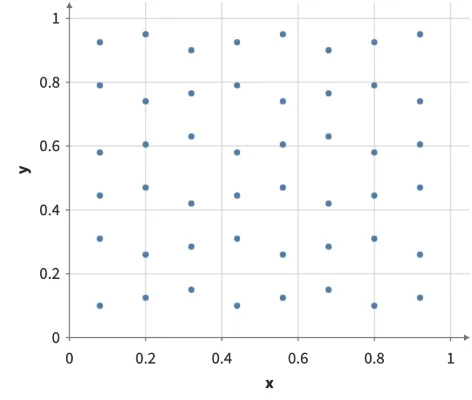
Draggable brush
Move a committed brush, clear it outside, and filter a sibling view through @brushed.
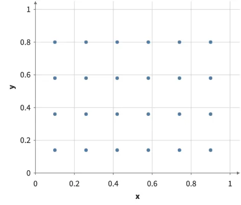
Explicit shared selection
Name one reusable selection, expose it as a virtual column, and share it across views.
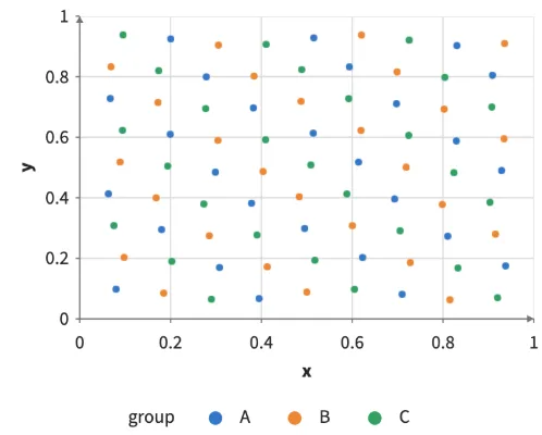
Multiple selection sets
Build two named selection sets in separate projections and inspect their overlap in a third view.
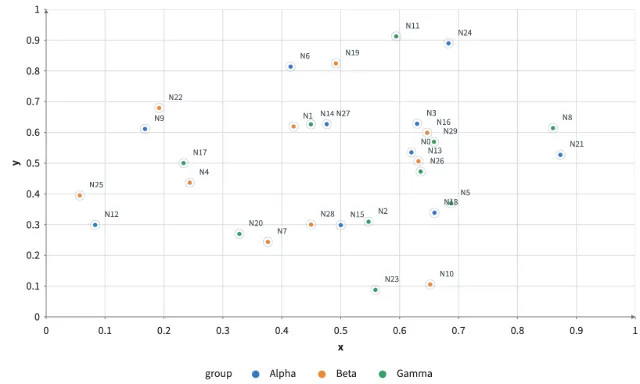
Interrupted keyed transitions
Interrupt keyed updates while points, halos, and labels use different fade timings and preserve interaction state.
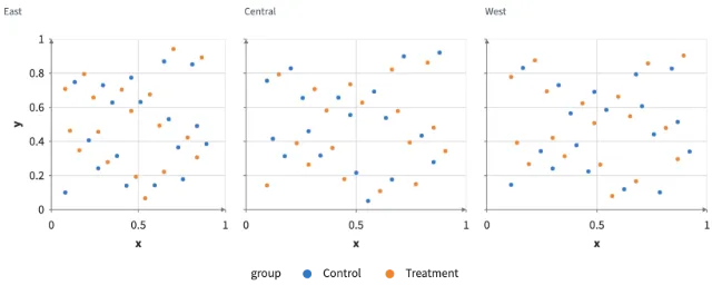
Faceted interaction state
Select, hover, and brush in linked facet cells while a detail plot consumes the shared keyed state.
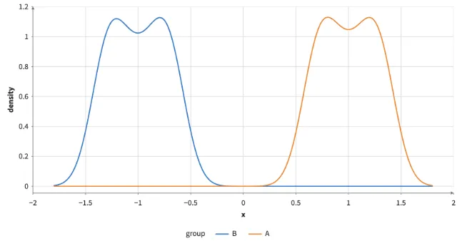
Density estimation
Grouped 1D and raster 2D Gaussian kernel density estimates.
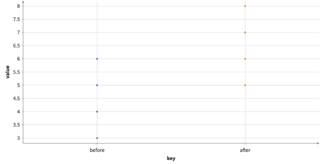
Pivot and fold
Reshape long and wide tables while retaining source identities.
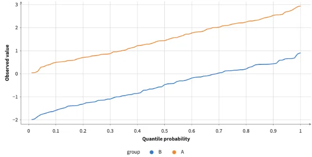
Quantiles and group summaries
Grouped quantile curves and each row's group mean and 90th percentile, all Calculate expressions.
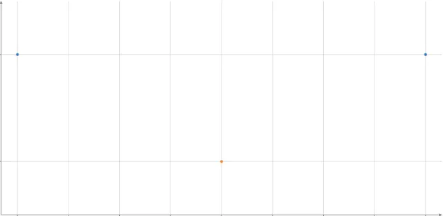
Categorical and datetime frames
Composable data scopes, coordinate frames, and shared navigation.
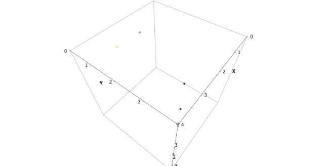
Three-dimensional axes
Composable data scopes, coordinate frames, and shared navigation.
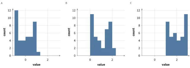
Facet settings
Composable data scopes, coordinate frames, and shared navigation.
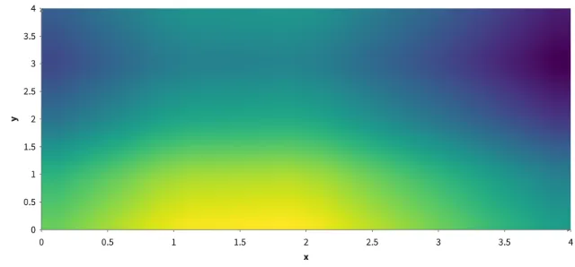
Bilinear grid
GPU-resident transforms with interactive controls.
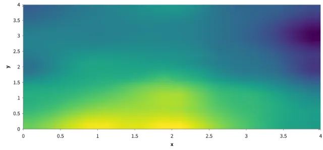
Scattered interpolation
GPU-resident transforms with interactive controls.
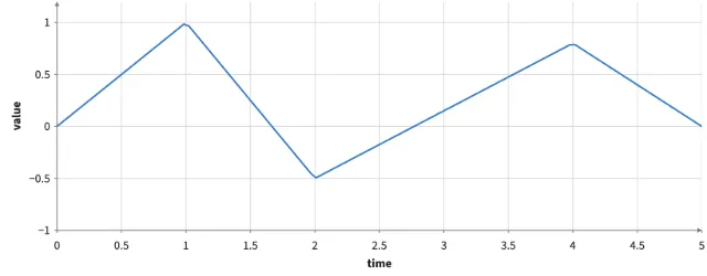
Signal interpolation
GPU-resident transforms with interactive controls.
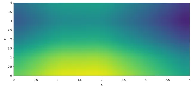
Time-varying field
GPU-resident transforms with interactive controls.
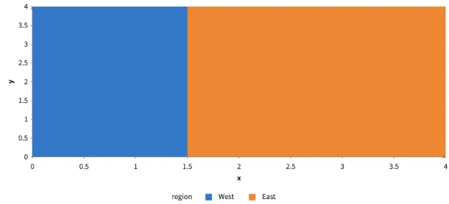
Categorical grid
GPU-resident transforms with interactive controls.
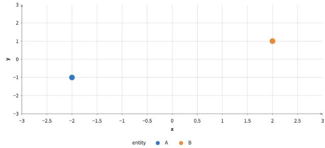
Entity motion
GPU-resident transforms with interactive controls.
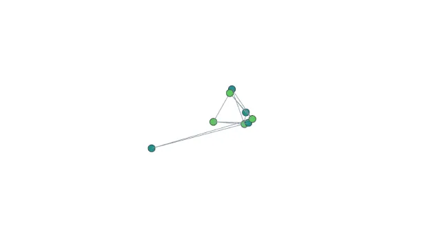
Force layout · 3D
GPU-resident transforms with interactive controls.
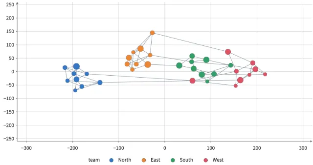
Layered forces
d3's forces by name, their strengths and targets from node columns.
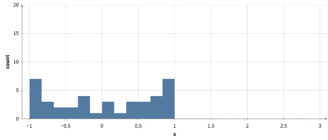
Inputs
A Select, a Playback and a Slider drive a Filter and a Bin by name; the options and a range are read from the data.
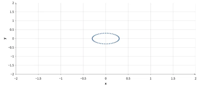
Springs
Simulate steps a ring of damped springs every 16 ms: Sliders set the stiffness and damping, Run pauses, Kick starts again, and a clicked point's spring pulls it out.
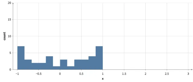
Filter and bin inputs
A Select with multiple=true of the species column's categories filters the rows, and a Slider sets the histogram's bin count.
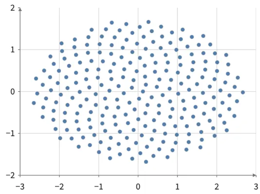
Linked views & minimap
Two views share a viewport. An external overview retains the full domain.
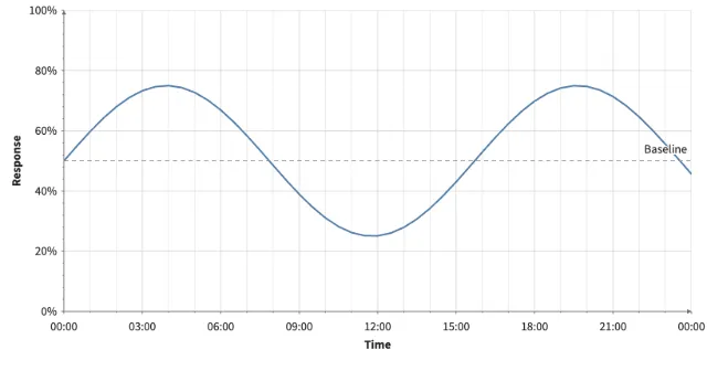
Axes & datetime
Calendar-aware labels, major/minor grids, reference rules, and axis-specific zoom.
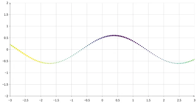
Animated points
Change targets during a transition. Data and appearance interpolate on the GPU.
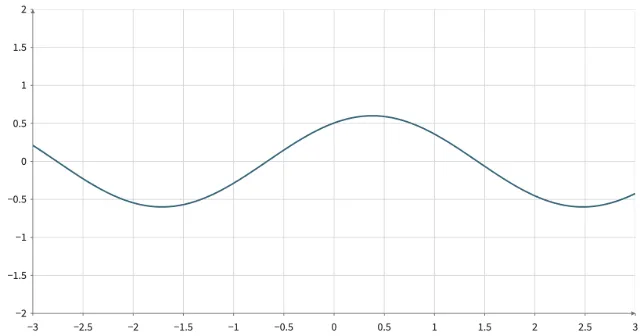
Animated line
Change targets during a transition. Data and appearance interpolate on the GPU.
Time
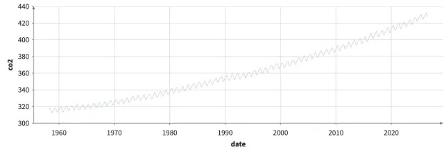
Calendar functions and a Playback over dates
Mauna Loa's monthly CO2: a Playback whose value is a date draws it a month at a time, four years a second, and month_name groups the seasonal cycle by calendar month.
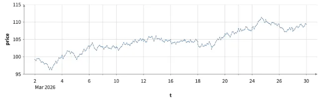
Market hours: an axis that skips weekends and nights
Half-hourly prices on an axis that leaves out weekends and the hours outside a 09:30 to 16:00 session in New York; the line runs on from each close to the next open, and a brush can span a break.
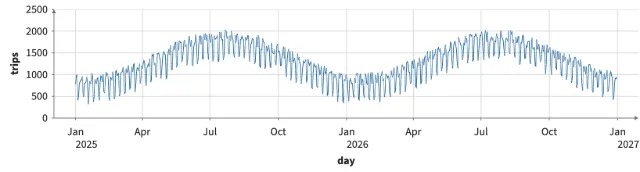
Days of the week and calendar months
Two years of daily trips: grouped by day_name into weekdays, Monday first, and binned by calendar month with Bin's interval, whose bars start and end at month boundaries.
Maps
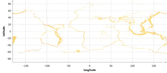
Earthquakes from a Parquet file
A Provider reads three of a Parquet file's five columns (ten years of USGS earthquakes, magnitude 4.5+) with HTTP range requests; the other two are never downloaded. Python reads the same columns with hm.Table.from_parquet.
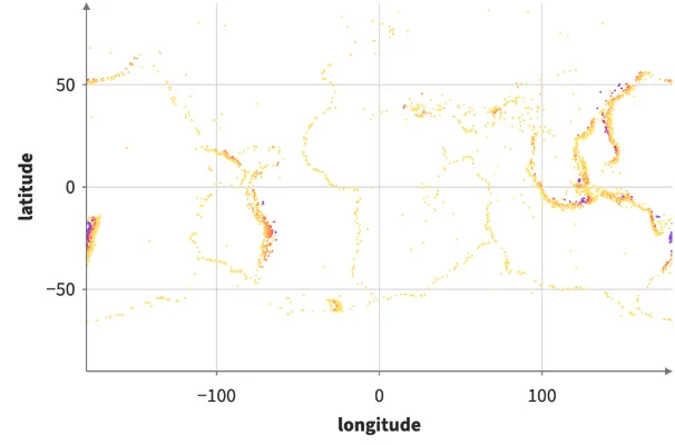
Earthquakes by year, loaded on demand
A Provider loads one year of real earthquakes (USGS, magnitude 4.5+) from a static CSV when the Year input changes. The previous year stays drawn until the next one arrives, a year already on screen loads nothing, and the Refresh button loads it again.
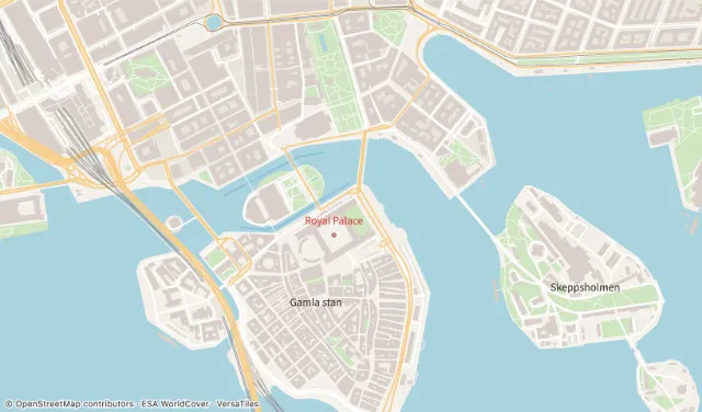
Vector tiles that follow the view
A VectorTile loads the tile named for a place at full detail, then, as you pan and zoom, the tiles the view shows (OpenStreetMap data as Mapbox Vector Tiles from VersaTiles), each drawn as soon as it arrives: water, parks, buildings, roads, railways and place names. Pick a place, a theme to recolor the basemap, hide layers (a hidden layer is never decoded), or turn Live off to keep only the named tile; the credit line is part of the plot and its exports.
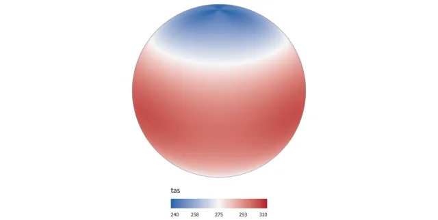
A gridded field on the globe, month by month
A grid table (month x latitude x longitude, one row per cell) holds a made-up surface temperature on 48 uneven latitudes. Slice through time blends the two months around a Playback's value on the GPU; the Heatmap places the latitudes by their coordinates.
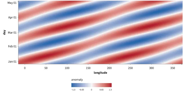
A Hovmöller diagram
Slice at one latitude of a time x latitude x longitude grid table leaves time against longitude: an anomaly travelling east is diagonal banding. The latitude is a slider.
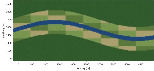
An RGB image from band columns
An Image's fill takes { r, g, b } columns, as every mark's RGB channel does: three satellite-style bands of a grid table (integers 0-255) make the image, placed by the grid's coordinates.
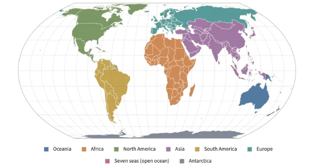
World map projections
equal-earth and natural-earth world maps, albers (conic equal-area) and albers-usa (the United States with Alaska and Hawaii as insets): each maps longitude and latitude jointly into one curved outline around its center, cut at its seam, with a graticule and outline instead of edge axes. Move the center to move the seam; click a country for the longitude and latitude under the pointer.
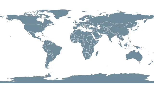
Country map
GPU maps with feature data and interaction.
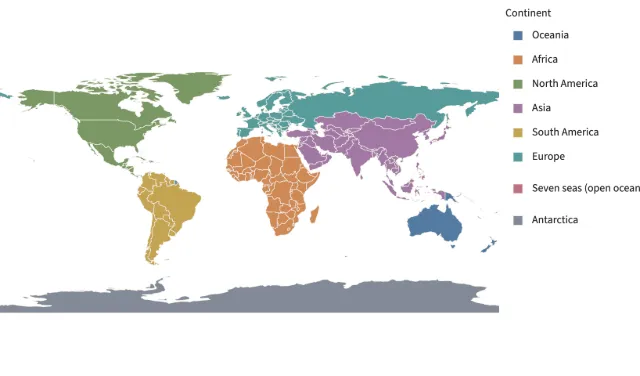
Categorical map
GPU maps with feature data and interaction.
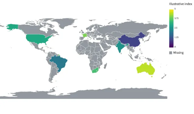
Joined choropleth
GPU maps with feature data and interaction.
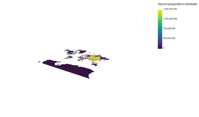
Projected extrusions
GPU maps with feature data and interaction.
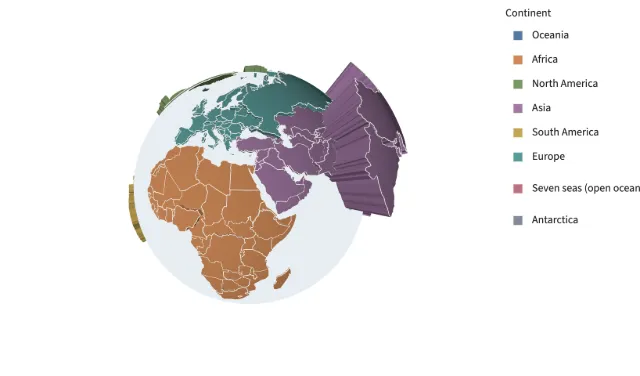
Globe extrusions
GPU maps with feature data and interaction.
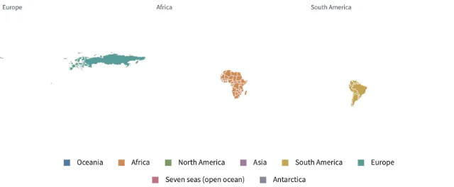
Filtered and faceted maps
GPU maps with feature data and interaction.
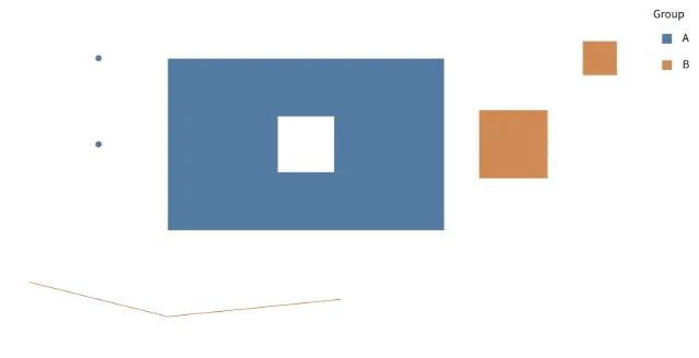
GeoJSON geometry
Feature picking, holes, and extruded regions.
Surfaces
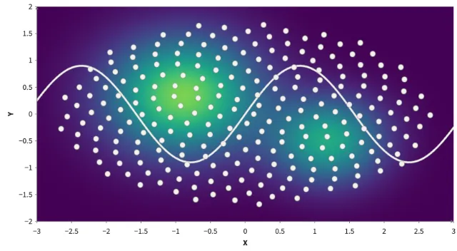
Interactive textures
Points and paths painted into a heatmap texture remain clickable on its surface.
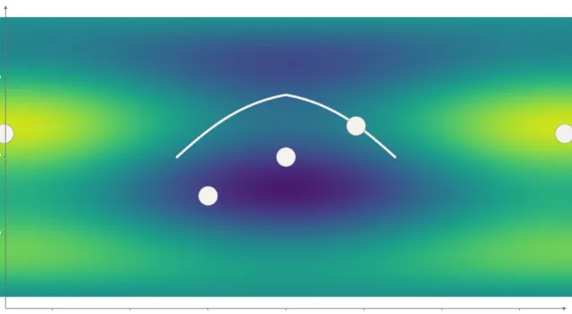
Spherical coordinates
Longitude–latitude data becomes a globe or a wrapping map, with a linked overview.
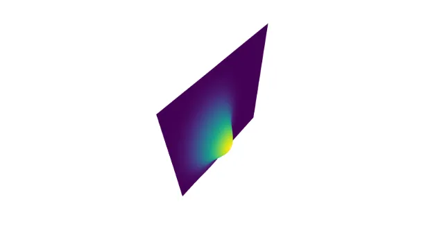
Animated surface
Change targets during a transition. Data and appearance interpolate on the GPU.
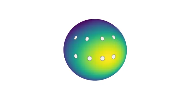
Animated globe
Change targets during a transition. Data and appearance interpolate on the GPU.