HMPlot
Composable plots for Svelte and Python.
HMPlot is an experimental visualization library built around three goals:
- A simple, declarative syntax for complex interactive scenes, including 3D.
- GPU-native data processing: jax-js arrays plot directly from the GPU, with no copy back to the CPU.
- Live plot customization, with publication-quality SVG and PDF export.
It is written in Svelte, with first-class Python support that includes inline rendering in notebooks. It was originally designed for real-time visualization of neural networks, as in these teaching demos.
A first plot
A simple example using the Palmer Penguins dataset.
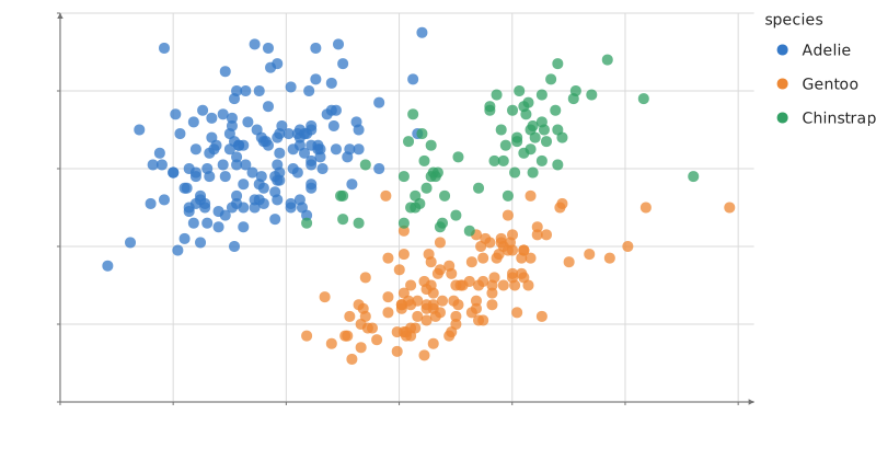
Static preview; loading the interactive plot
<script>
  import { autoType, csvParse } from "d3";
  import { Legend, Plot, Points } from "hmplot";
  import csv from "./penguins.csv?raw";

  // Palmer penguins (CC0): https://allisonhorst.github.io/palmerpenguins/
  // Two penguins have no bill measurements: skip them.
  const penguins = csvParse(csv, autoType)
    .filter((p) => p.bill_length_mm !== null && p.bill_depth_mm !== null);
</script>

<Plot data={penguins} height={420} axes2d
  x={{ label: "Bill length (mm)", grid: "major" }} y={{ label: "Bill depth (mm)", grid: "major" }}>
  <Points x="bill_length_mm" y="bill_depth_mm" fill="species" opacity={0.75} />
  <Legend channel="fill" />
</Plot>
Install
HMPlot 0.1.0-alpha.1 is an alpha release: the API may still change. It is not on PyPI or npm yet; install it from its GitHub release. Report problems on GitHub.
Python
Python 3.11 or later, in the environment of your notebook's kernel:
pip install https://github.com/gabehope/HMPlot/releases/download/v0.1.0-alpha.1/hmplot-0.1.0a1-py3-none-any.whlSvelte
Svelte 5; npm also installs the peer dependencies, three.js and Threlte:
npm install https://github.com/gabehope/HMPlot/releases/download/v0.1.0-alpha.1/hmplot-0.1.0-alpha.1.tgzInteractive rendering requires WebGPU, in the browser or the notebook's webview.
Gallery
Statistics, linked views, graphs, maps and 3D scenes, each with its source.
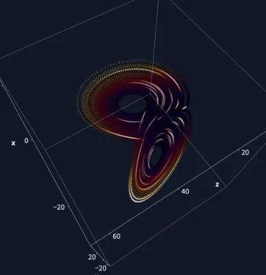
Lorenz attractor
Sixty thousand Runge-Kutta steps of the Lorenz system trace its butterfly; on the GPU every point then moves on at the Rayleigh number you drag, collapsing onto two fixed points below about 24.7. A glowing 3D orbit with sparks that run along it in time order (evaluated on the GPU from @time), linked to the butterfly projection: brush a region and the 3D view keeps only those points lit while a speed histogram counts them.
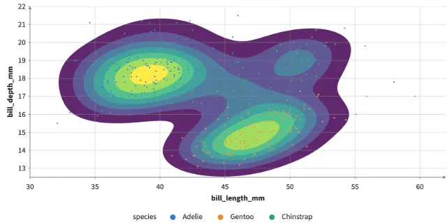
Density contours
The density of penguins' bill length against depth as filled bands, contour lines or both, on the GPU: Density, then Contour's marching squares.
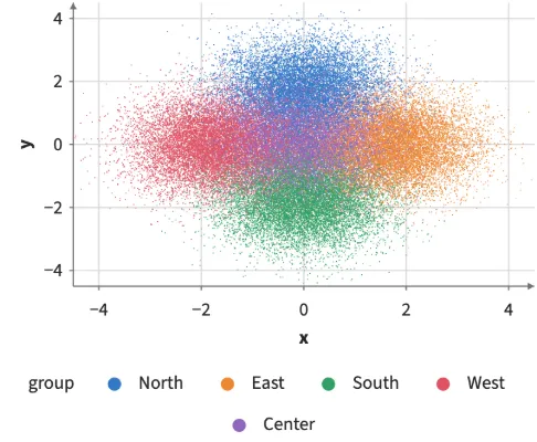
Brushed distributions
Shift-drag to brush 60,000 points in five clusters; violins and box plots of each group's values are recomputed from the brushed rows on every move, with no GPU kernels compiled while dragging.
Large force graph
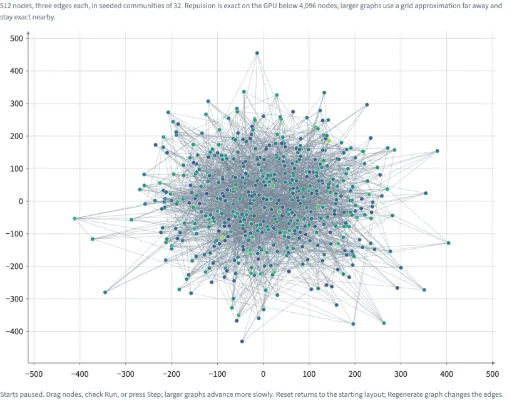
Explore seeded graphs of 64 to 10,000 nodes, thin edges, dragging, and a linked overview in 2D or 3D.
Earthquakes beneath the globe
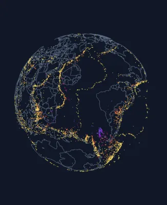
Every earthquake of magnitude 4.5+ in 2024 (6,397 events, USGS) placed at its true depth inside a see-through globe, where deep quakes trace subducting slabs; a slider exaggerates the depths. Brush a region on the map and a period on the timeline; the brushes combine, the globe keeps the matching quakes lit, and a log-scale histogram shows the Gutenberg–Richter law.
Streamgraph
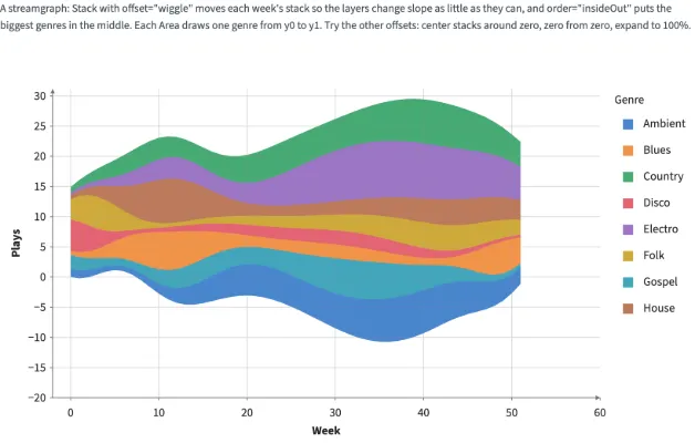
Stack with offset="wiggle" and order="insideOut": each week's stack moves so the layers change slope as little as they can, the biggest genres in the middle, and an Area per genre draws it. The controls switch the offset and the order. Area transitions animate by default; the Animate control can turn them off.
Clustered heatmap
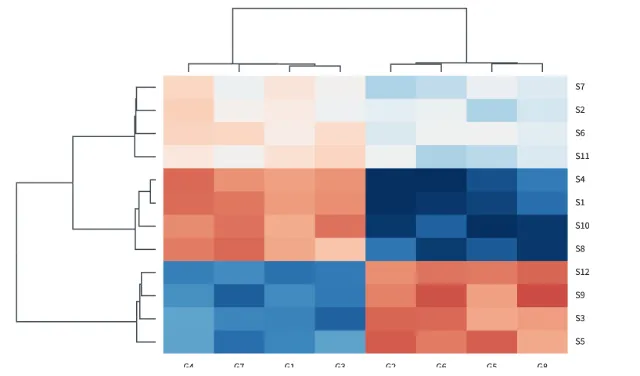
A heatmap sorted by two dendrograms, as seaborn's clustermap: Tree mode="cluster" draws each precomputed linkage to scale by its merge heights, in Frames that share the heatmap's rows and columns, and labels the leaves by their order.
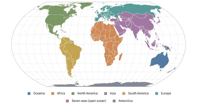
World map projections
equal-earth and natural-earth world maps, albers (conic equal-area) and albers-usa (the United States with Alaska and Hawaii as insets): each maps longitude and latitude jointly into one curved outline around its center, cut at its seam, with a graticule and outline instead of edge axes. Move the center to move the seam; click a country for the longitude and latitude under the pointer.