Earthquakes beneath the globe
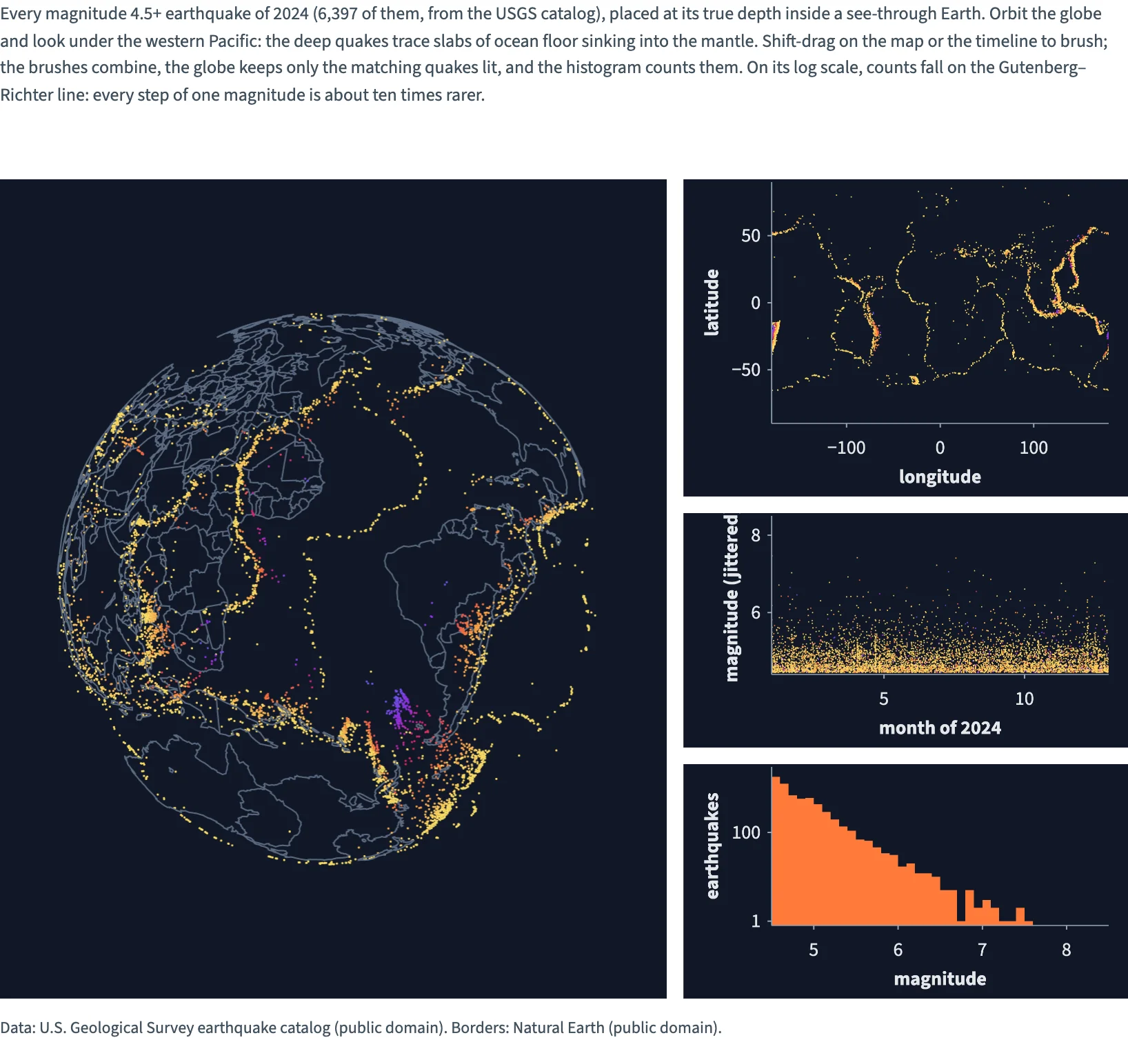
Every earthquake of magnitude 4.5+ in 2024 (6,397 events, USGS) placed at its true depth inside a see-through globe, where deep quakes trace subducting slabs; a slider exaggerates the depths. Brush a region on the map and a period on the timeline; the brushes combine, the globe keeps the matching quakes lit, and a log-scale histogram shows the Gutenberg–Richter law.
Static preview; loading the interactive plot
<script>
  import { InputContext, Slider, Theme, themes, Data, Plot, GeoJSON, Calculate, Points, Rect, continuous, col, input, multiply } from "hmplot";
import { Bin } from "hmplot/stats";
  import quakes from "./quakes-2024.json";
  import countries from "./countries.json";

  // Every earthquake of magnitude 4.5 or more in 2024 (USGS), placed at its true depth inside a
  // see-through globe: the slabs where plates sink show as sheets of deep (violet) quakes. The
  // slider exaggerates the depths; shift-drag on the map or the timeline to brush.

  // Magnitudes come rounded to 0.1, which draws the timeline as stripes: spread each by a fixed
  // pseudo-random amount within 0.05, for display only.
  const jittered = quakes.mag.map((mag, i) => {
    const noise = Math.sin(i * 12.9898) * 43758.5453;
    return mag + 0.1 * (noise - Math.floor(noise) - 0.5);
  });
  // Shallow quakes are hot yellow; the deepest, 700 km down, violet.
  const depthColors = continuous({ domain: [0, 700], colormap: ["#ffe066", "#ff7b39", "#e0245e", "#8e2de2", "#4361ee"] });
  const magnitudes = Array.from({ length: 41 }, (_, i) => Math.round((4.5 + i * 0.1) * 10) / 10);
  // A spherical position is [longitude, latitude, offset], at radius 1 + offset: the depth as a
  // fraction of Earth's radius, times the slider's exaggeration. Computed on the GPU, so a new
  // value reruns the globe's positions only.
  const radius = multiply(multiply(col.depth, input.exaggeration), -1 / 6371);
  // Shared side margins align the detail panels in this CSS layout and the Python version.
  const panelMargins = { axisMarginLeft: 64, axisMarginRight: 14 };
</script>

<InputContext>
  <p>Every magnitude 4.5+ earthquake of 2024 (6,397 of them, from the USGS catalog), placed at its true depth inside a see-through Earth. Orbit the globe and look under the western Pacific: the deep quakes trace slabs of ocean floor sinking into the mantle. Shift-drag on the map or the timeline to brush; the brushes combine, the globe keeps only the matching quakes lit, and the histogram counts them. On its log scale, counts fall on the Gutenberg–Richter line: every step of one magnitude is about ten times rarer.</p>
  <Slider name="exaggeration" label="Depth exaggeration" min={1} max={6} step={0.1} value={4} format=".1f" />
  <Theme value={themes.dark}>
    <Data value={{ ...quakes, jittered }}>
      <div class="row">
        <!-- A fixed offset domain keeps the slider from changing the globe's extent. The camera
             looks at the Pacific, where the Ring of Fire and the deep slabs are. -->
        <div class="main">
          <Plot coordinates="spherical" type="3d-y-up" height={594} globeBackground={false}
            z={{ domain: [-0.7, 0] }} cameraPosition={[1.1, 0.9, -3.0]}>
            <GeoJSON data={countries} color="#5b6b82" width={1}  fill={null} />
            <Calculate columns={{ radius }}>
              <Points x="lon" y="lat" z="radius" fill="depth" fillScale={depthColors} size={1.5}
                respond="brushed" legend={false} />
            </Calculate>
          </Plot>
        </div>
        <div class="side">
          <Plot {...panelMargins} height={230} axes2d x={{ domain: [-180, 180], label: "longitude" }} y={{ domain: [-90, 90], label: "latitude" }}>
            <Points x="lon" y="lat" fill="depth" fillScale={depthColors} size={1} brush respond="brushed" legend={false} />
          </Plot>
          <Plot {...panelMargins} height={170} axes2d x={{ domain: [1, 13], label: "month of 2024" }} y={{ domain: [4.4, 8.5], label: "magnitude (jittered)" }}>
            <Points x="month" y="jittered" fill="depth" fillScale={depthColors} size={1} brush respond="brushed" legend={false} />
          </Plot>
          <Plot {...panelMargins} height={170} axes2d x={{ domain: [4.5, 8.5], label: "magnitude" }}
            y={{ domain: [0.8, 3000], transform: "log", label: "earthquakes" }}>
            <!-- Dim: every quake. Bright: the brushed ones (all of them with no brush). -->
            <Bin x="mag" bins={magnitudes}>
              <Rect x0="x0" x1="x1" y0={0.8} y1="count" fill="#3b3363" legend={false} />
            </Bin>
            <Bin x="mag" bins={magnitudes} weight="@brushed">
              <Rect x0="x0" x1="x1" y0={0.8} y1="count" fill="#ff7b39" legend={false} />
            </Bin>
          </Plot>
        </div>
      </div>
    </Data>
  </Theme>
  <small>Data: U.S. Geological Survey earthquake catalog (public domain). Borders: Natural Earth (public domain).</small>
</InputContext>

<style>
  /* Three fifths and two fifths, 12 px apart; one column once the side would be narrower than
     286 px. Python's Row(widths=[3, 2], wrap=True, min_width=286, gap=12) lays them out the same. */
  .row { display: flex; flex-wrap: wrap; gap: 12px; margin: 12px 0; }
  .main { flex: 3 1 429px; min-width: 0; }
  .side { flex: 2 1 286px; min-width: 0; display: flex; flex-direction: column; gap: 12px; }
</style>