Lorenz attractor
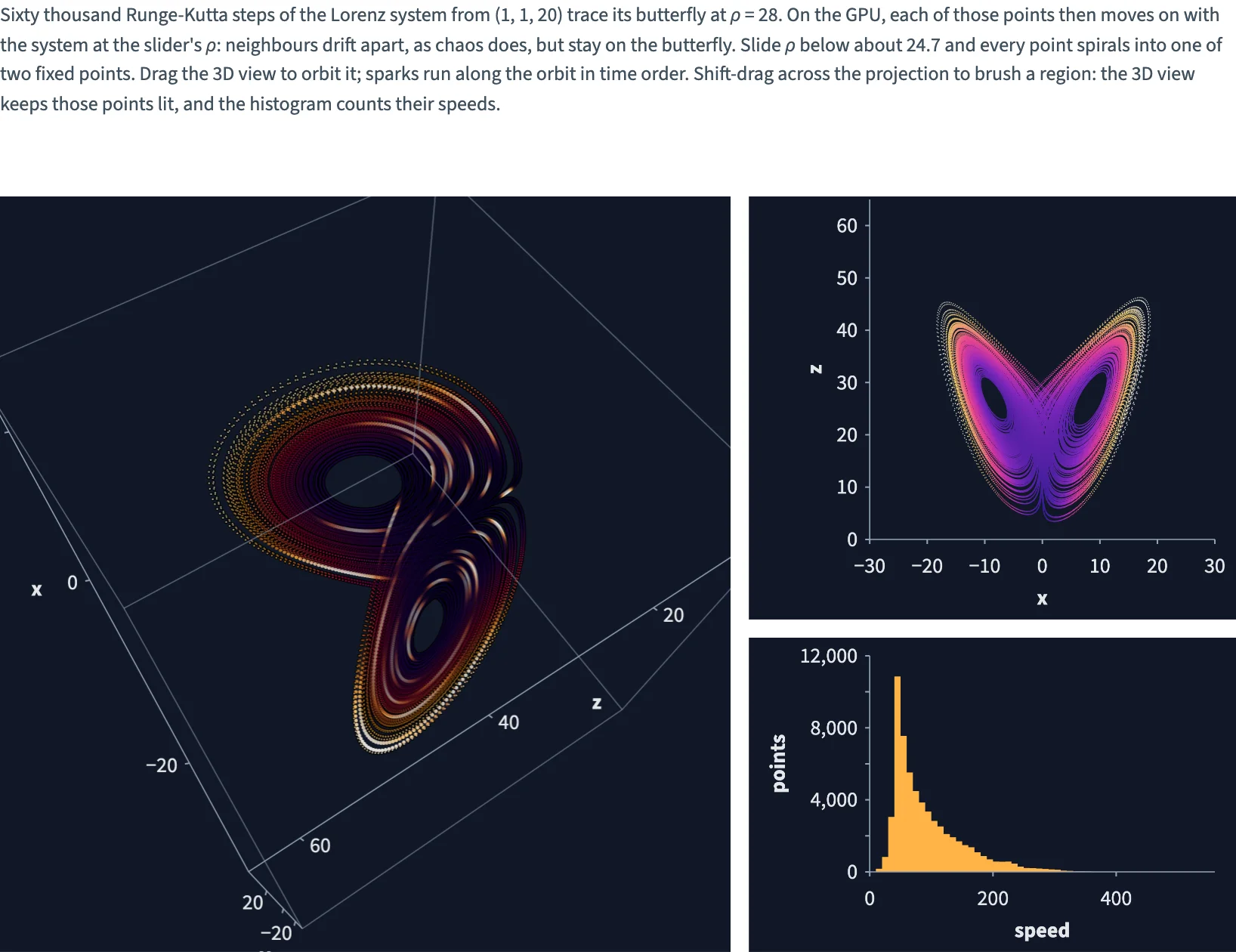
Sixty thousand Runge-Kutta steps of the Lorenz system trace its butterfly; on the GPU every point then moves on at the Rayleigh number you drag, collapsing onto two fixed points below about 24.7. A glowing 3D orbit with sparks that run along it in time order (evaluated on the GPU from @time), linked to the butterfly projection: brush a region and the 3D view keeps only those points lit while a speed histogram counts them.
Static preview; loading the interactive plot
<script>
  import { InputContext, Slider, Theme, themes, Data, Simulate, Calculate, Plot, Points, Rect, continuous, input, prev, col, view, add, subtract, multiply, divide, sqrt, square, exp, cos, where, greater, less, logical_or } from "hmplot";
import { Bin } from "hmplot/stats";

  // The Lorenz attractor: sixty thousand Runge-Kutta steps from (1, 1, 20) at rho = 28 trace the
  // butterfly. On the GPU, each of those points then moves on with the system at the slider's rho
  // (Simulate: a midpoint step of 0.02 every 16 ms); a new rho starts again from the butterfly.
  const STEPS = 60000, DT = 0.003;
  const f = (x, y, z) => [10 * (y - x), x * (28 - z) - y, x * y - (8 / 3) * z];

  const orbit = { x: [], y: [], z: [], t: [] };
  let x = 1, y = 1, z = 20;
  for (let i = 0; i < STEPS; i++) {
    const a = f(x, y, z);
    const b = f(x + DT / 2 * a[0], y + DT / 2 * a[1], z + DT / 2 * a[2]);
    const c = f(x + DT / 2 * b[0], y + DT / 2 * b[1], z + DT / 2 * b[2]);
    const d = f(x + DT * c[0], y + DT * c[1], z + DT * c[2]);
    x += DT / 6 * (a[0] + 2 * b[0] + 2 * c[0] + d[0]);
    y += DT / 6 * (a[1] + 2 * b[1] + 2 * c[1] + d[1]);
    z += DT / 6 * (a[2] + 2 * b[2] + 2 * c[2] + d[2]);
    orbit.x.push(x); orbit.y.push(y); orbit.z.push(z);
    orbit.t.push(i / (STEPS - 1));
  }

  // The same system as expressions, at the slider's rho.
  const lorenz = (x, y, z) => [
    multiply(10, subtract(y, x)),
    subtract(multiply(x, subtract(input.rho, z)), y),
    subtract(multiply(x, y), multiply(8 / 3, z)),
  ];
  const H = 0.02;
  const [px, py, pz] = [prev("x"), prev("y"), prev("z")];
  const [kx, ky, kz] = lorenz(px, py, pz);
  const [mx, my, mz] = lorenz(add(px, multiply(H / 2, kx)), add(py, multiply(H / 2, ky)), add(pz, multiply(H / 2, kz)));
  // A point that has come to rest on a fixed point (speed below 2) leaves the view (x = 1e6) and
  // stays there: thousands of points blended on one spot would slow every frame.
  const rest = logical_or(greater(px, 1e5), less(add(add(square(kx), square(ky)), square(kz)), 4));
  const flow = {
    x: where(rest, 1e6, add(px, multiply(H, mx))),
    y: where(rest, py, add(py, multiply(H, my))),
    z: where(rest, pz, add(pz, multiply(H, mz))),
  };
  const [vx, vy, vz] = lorenz(col.x, col.y, col.z);
  const speed = sqrt(add(add(square(vx), square(vy)), square(vz)));

  // One ramp for every view, slow (deep violet) to fast (white-hot).
  const glow = continuous({ domain: [0, 320], colormap: ["#3a2a80", "#7a36b4", "#e8457a", "#ffb347", "#fff6d8"] });
  // Additive blending adds nothing for black: sparks fade from black to white-hot at their peak.
  const sparkRamp = continuous({ domain: [0, 1], colormap: ["#000000", "#ff9d3c", "#fff8e8"] });
  // Forty sparks: a narrow bump on every cycle of a phase that the clock moves along the orbit.
  const phase = multiply(6.283185, subtract(multiply(40, col.t), divide(view.time, 2500)));
  const spark = exp(multiply(400, subtract(cos(phase), 1)));
  const bins = Array.from({ length: 57 }, (_, i) => i * 10);
  // Shared side margins align the detail panels in this CSS layout and the Python version.
  const panelMargins = { axisMarginLeft: 80, axisMarginRight: 14 };
</script>

<InputContext>
  <p>Sixty thousand Runge-Kutta steps of the Lorenz system from (1, 1, 20) trace its butterfly at <em>ρ</em> = 28. On the GPU, each of those points then moves on with the system at the slider's <em>ρ</em>: neighbours drift apart, as chaos does, but stay on the butterfly. Slide <em>ρ</em> below about 24.7 and every point spirals into one of two fixed points. Drag the 3D view to orbit it; sparks run along the orbit in time order. Shift-drag across the projection to brush a region: the 3D view keeps those points lit, and the histogram counts their speeds.</p>
  <Slider name="rho" label="Rayleigh number ρ" min={12} max={35} step={0.1} value={28} />
  <Theme value={themes.dark}>
    <Data value={orbit}>
      <Simulate initial={{ x: "x", y: "y", z: "z" }} update={flow} reset={input.rho} step={16}>
        <Calculate columns={{ speed }}>
          <div class="row">
            <div class="main">
              <!-- The Lorenz z axis points up, so it maps to the plot's vertical y. -->
              <Plot type="3d" axes3d height={500} antialias="off" toneMapping={4} cameraPosition={[-70, 45, 160]}
                x={{ domain: [-30, 30], label: "x" }} y={{ domain: [0, 65], label: "z" }} z={{ domain: [-35, 35], label: "y" }}>
                <Points x="x" y="z" z="y" fill="speed" fillScale={glow} size={1.25} opacity={0.45}
                  blend="additive" respond="brushed" legend={false} />
                <Points x="x" y="z" z="y" fill={spark} fillScale={sparkRamp} size={2.5} blend="additive"
                  respond={false} legend={false} />
              </Plot>
            </div>
            <div class="side">
              <Plot {...panelMargins} height={280} axes2d antialias="off" toneMapping={4} x={{ domain: [-30, 30], label: "x" }} y={{ domain: [0, 65], label: "z" }}>
                <Points x="x" y="z" fill="speed" fillScale={glow} size={0.75} blend="additive"
                  brush respond="brushed" legend={false} />
              </Plot>
              <Plot {...panelMargins} height={208} axes2d antialias="off" x={{ domain: [0, 560], label: "speed" }} y={{ label: "points" }}>
                <!-- Dim: every point. Bright: the brushed ones (all of them with no brush). -->
                <Bin x="speed" {bins}>
                  <Rect x0="x0" x1="x1" y0={0} y1="count" fill="#3b3363" legend={false} />
                </Bin>
                <Bin x="speed" {bins} weight="@brushed">
                  <Rect x0="x0" x1="x1" y0={0} y1="count" fill="#ffb347" legend={false} />
                </Bin>
              </Plot>
            </div>
          </div>
        </Calculate>
      </Simulate>
    </Data>
  </Theme>
</InputContext>

<style>
  /* Three fifths and two fifths, 12 px apart; one column once the side would be narrower than
     286 px. Python's Row(widths=[3, 2], wrap=True, min_width=286, gap=12) lays them out the same. */
  .row { display: flex; flex-wrap: wrap; gap: 12px; margin-top: 12px; }
  .main { flex: 3 1 429px; min-width: 0; }
  .side { flex: 2 1 286px; min-width: 0; display: flex; flex-direction: column; gap: 12px; }
</style>