Tree
A rooted tree layout of an edge table, as a tidy tree, an icicle or a dendrogram.
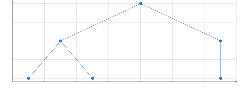
Static preview; loading the interactive plot
import hmplot as hm

data = {"source": ["root", "root", "a", "a", "b"], "target": ["a", "b", "a1", "a2", "b1"]}
with hm.Plot(data=data, height=300) as plot:
    with hm.GraphData(source="source", target="target"):
        with hm.Tree(root="root"):
            with hm.Edges():
                hm.Segments(start="start", end="end")
            with hm.Nodes():
                hm.Points(position="position")
plot
Usage
Provides Nodes and Edges scopes with parent, depth, degree, order, positions, and endpoints. Drops unreachable nodes and non-tree edges. Default traversal is undirected, orientation down, and spacing 1. directed follows source-to-target edges. A missing root is an error.
All modes honor directed: true follows outgoing edges and shows a subtree, false traverses either way and reroots the reachable component. The root has depth zero, and Edges publish the child node’s depth, even when an original edge points toward the root. Explicit node tables retain selection and keyed animation identity while unreachable nodes are omitted. Automatic bounds update when layout geometry changes; explicit domains remain fixed.
Nodes also publish parentPosition, parentX and parentY, plus parentX0/parentX1/parentY0/parentY1 in partition mode. Roots have NaN parent coordinates. These support enter/exit animation: x={animate(col.x, {enter: col.parentX, exit: col.parentX})}. New rows read their new parent’s coordinates; departing rows read their previous parent’s coordinates.
root can be a scalar reduction expression over the original node table, including its selection. See Zoomable sunburst for declarative focus and Expandable tree for collapse, depth filtering and layout-owned transitions.
In mode="partition", visualMargin insets the published node bounds to create visible gaps between sibling rectangles and depth bands. It defaults to zero, and the node x/y centers stay fixed.
Every mode publishes order on its nodes: each leaf’s place among the leaves, left to right (0, 1, 2, …), and NaN for inner nodes, so marks placed by it skip them. A nodes table may not have its own order column.
Requires graph data from GraphData. Outputs are visible to children only. Transforms retain the previous complete result while an update prepares. To let the viewer change a setting, read an input in it: orientation={input("orientation")} (Python orientation=hm.input.orientation), where orientation is a Select of "down", "up", "left" and "right".
Dendrograms
Partition widths and heights can be zero. layerHeight accepts a number, node-table column or expression, with each child’s band starting at its parent’s end. tween() in nodeWidth and layerHeight runs before layout on the plot clock. With a stable topology, tweening unwanted subtree weights and ancestor heights to zero shrinks them coherently; restoring the values grows them. Filter zero-area nodes after layout and draw the moving geometry directly, without another mark transition. See Zoomable sunburst.
mode="cluster" lays a tree out as d3.cluster does: every leaf at the same level, one siblingSpacing apart in order (leaf k at k), and each parent centered over its children (their mean). The leaves sit at 0 along the tree and the root at the far end. Without height, a node sits 1 + its tallest child from the leaves (times depthSpacing). With height, a column of the nodes table (or an expression over it), each node sits at its merge height, drawn to scale as scipy’s dendrogram draws it: y is the height in "down", -height in "up", x is the height in "left" and -height in "right". Leaves take height 0 (a missing value reads as 0); a merge needs a finite height, at least its children’s, and Tree names the node otherwise. Only nodes reachable from the root are published.
Draw the links with Segments and a step curve for right-angle elbows: curve="step-after" (across, then along) for "down" and "up", and curve="step-before" for "left" and "right". In a polar Plot or Frame, "up" with step-after draws arcs, then radial lines; a baseRadius equal to the root’s height puts the root at the center.
A clustered heatmap sorts its rows (or columns) in the order of the leaves, one unit per leaf, and puts each dendrogram in a Frame beside it whose leaf axis has the domain [-0.5, n - 0.5] over the heatmap’s n rows, so leaf k sits at the center of row k. Nodes can label the leaves with y="order" (or x="order").
Tree takes precomputed trees; it does not cluster. In Python, hm.linkage_table(Z, labels) turns a scipy linkage matrix into the tables below, and scipy.cluster.hierarchy.leaves_list(Z) is the leaf order. In JavaScript, turn merge rows [a, b, height] (scipy’s convention: leaves 0 to n - 1, merge i makes node n + i) into an edge table and a nodes table:
function linkageTable(merges, labels) {
  const n = labels.length, edges = { source: [], target: [] };
  const nodes = { id: labels.map((_, i) => i), label: [...labels], height: labels.map(() => 0) };
  merges.forEach(([a, b, height], i) => {
    edges.source.push(n + i, n + i); edges.target.push(a, b);
    nodes.id.push(n + i); nodes.label.push(null); nodes.height.push(height);
  });
  // The leaves left to right, as mode="cluster" places them (its order column).
  const leaves = [], stack = [2 * n - 2];
  while (stack.length) {
    const node = stack.pop();
    if (node < n) leaves.push(node); else stack.push(merges[node - n][1], merges[node - n][0]);
  }
  return { edges, nodes, root: 2 * n - 2, leaves };
}<GraphData nodes={rows.nodes} edges={rows.edges}>
<Tree root={rows.root}
mode="cluster" height="height" orientation="down">
<Edges><Segments start="start" end="end" curve="step-after" /></Edges>
</Tree>
</GraphData>A d3 hierarchy converts the same way: root.links() lists each parent with its children, in order, for the edge table, and the nodes table takes each node’s merge height from its data.
See the complete example.
Tree layout animation
Tree offers compact CPU tidy, GPU tidy-approx (horizontal intervals per subtree),
GPU partition, and CPU cluster. GPU modes cache topology by node IDs/order, source/target
columns, root and direction. Width/height changes reuse structural buffers. Partition uses
leaf prefix sums; root-path accumulation uses logarithmic pointer-jumping passes. Approximate
and fixed-width subtree sizing uses ordered depth passes, so very deep trees cost more.
CPU tidy can consume moving inputs too, but reads numeric values and lays out on the host.
edgeLength (Python edge_length) reads a nonnegative edge-table column or expression.
Tidy modes accumulate lengths along root paths, multiplied by depthSpacing; siblings can
have unequal lengths. Partition uses per-node layerHeight; cluster uses merge heights.
Put visibility on Tree’s where, not a Filter after Nodes, when branches should reflow.
It reads the node table and disconnects descendants of hidden nodes; the root remains present.
Tree’s enter and exit specify nonnegative numeric nodeWidth, layerHeight, and edgeLength contributions (omitted endpoints are zero). animationDuration and animationEasing control these lifecycle transitions. Initial mounting rests at the target.
In Python, nested keys are node_width, layer_height, and edge_length.
Departing nodes and edges remain until their contributions land; new rows start at enter
values. Interrupted membership transitions continue from their current contribution. presence on Nodes and Edges ranges from zero to one, so opacity="presence" fades marks
with their branch. Incoming tween() expressions remain ordinary numeric inputs with their
own timing; they do not declare layout entry/exit. Draw moving geometry directly without
another mark animation or bounds animation. Cluster does not support layout lifecycle.
Changing the root or reparenting a surviving node switches topology discretely; it does not
retain both parents. Use a fixed root with tweened weights/heights for continuous zoom, as in
the sunburst example. Structural changes may compile a new GPU plan.
Source validation and membership updates may read data once; GPU numeric layout does not read coordinates back each frame. Rendering, bounds, picking and export retain their existing readbacks. See Expandable tree and Sunburst.