Sankey
A flow diagram layout, with nodes in columns and links as thick as their values.
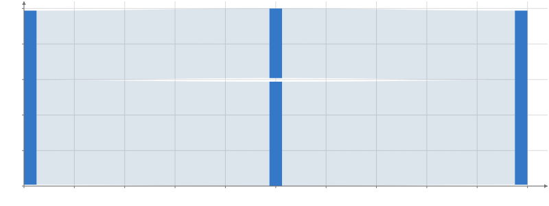
Static preview; loading the interactive plot
import hmplot as hm

data = {"source": ["in", "in", "a", "b"], "target": ["a", "b", "out", "out"], "value": [3, 2, 3, 2]}
with hm.Plot(data=data, height=300) as plot:
    with hm.GraphData(source="source", target="target"):
        with hm.Sankey(value="value"):
            with hm.Edges():
                hm.Flow(start_lower="startLower", end_lower="endLower",
                        start_upper="startUpper", end_upper="endUpper")
            with hm.Nodes():
                hm.Rect(x0="x0", x1="x1", y0="y0", y1="y1")
plot
Usage
Sankey consumes GraphData and lays out nonnegative flows in an acyclic directed graph. Nodes expose x0, x1, y0, y1, x, y, position, depth, and throughput. Edges expose four attachment corners for Flow, plus the original edge columns. Explicit GraphData node tables can include isolated nodes.