stats.Bin
Counts the rows in each interval of x (a histogram), or in each cell of an x-y or x-y-z grid.
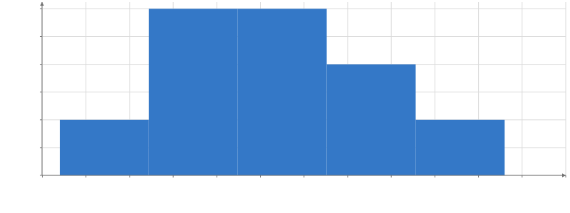
Static preview; loading the interactive plot
import hmplot as hm

data = {"value": [1.2, 2.5, 2.9, 3.1, 3.4, 3.8, 4.2, 4.4, 5.1, 6.3]}
with hm.Plot(data=data, height=300, axes2d=True) as plot:
    with hm.stats.Bin(x="value", bins=5):
        hm.Rect(x0="x0", x1="x1", y0=0, y1="count")
plot
Usage
Outputs centers, lower/upper bounds per dimension, count, and columns: reduction expressions as in Group (columns={{ mean_y: mean("y") }}), missing for an empty bin. Defaults to 30 bins; bins may instead supply explicit edges. Aggregate mode includes empty rectangular bins; assign mode keeps original rows. Bins are half-open except for the last upper boundary.
For a histogram over x alone (or y alone), normalization gives each bin its bar along the other axis: y0 (0), y1 and y hold its count ("count"), its share of all the rows ("proportion"), or that share divided by the bin’s width ("density"); binning y gives x0, x1 and x instead. So <Rect x0="x0" x1="x1" y0="y0" y1="y1" /> draws the bars either way round, as Histogram does.
bins also takes a rule name — "auto", "sturges", "fd", or "scott", computed from the data exactly as numpy does — or an expression evaluated against this transform’s input, such as power(count(col.x), 0.5). Either way the count is resolved before binning, and re-resolved whenever the data changes. Changing a bin count changes the number of rows, so marks snap to the new bins rather than animating between them.
Inside a Facet, bins are shared across the cells by default, so a rule name or an expression is resolved once over the rows of every cell together and each cell gets the same edges. Set sharedBins={false} to resolve the count per cell, against that cell’s rows.
To let the viewer change a setting, read an input in it: bins={input("bins")} (Python bins=hm.input.bins), where bins is a Slider.