Regression
A least-squares fit of y on x, sampled across x, with its confidence band.
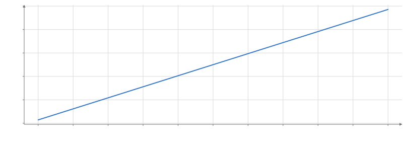
Static preview; loading the interactive plot
import hmplot as hm

data = {"x": [1, 2, 3, 4, 5, 6], "y": [2, 3, 5, 4, 6, 7]}
with hm.Plot(data=data, height=300, axes2d=True) as plot:
    with hm.Regression(x="x", y="y"):
        hm.Line(x="x", y="y")
plot
Usage
A least-squares fit of y on x over the rows shown, sampled at samples evenly spaced x values across the fitted rows (or extent), with a confidence band for the mean response from Student’s t at n − k − 1 degrees of freedom. method picks the model: linear, poly (order 1 to 6), log (y on ln x), exp (ln y on x) or pow (ln y on ln x); exp and pow bands are asymmetric.
The fit runs on the GPU, so a Filter or a brush above it refits as it moves. The handle’s fit() resolves to a RegressionFit: the method and order, the coefficients from the constant up (of response, y or ln y, in variable, x or ln x), r2, the residual sum of squares rss, the rows fitted n and the degrees of freedom df; null before the first run. Requires a Data scope; outputs x, y, lower and upper to its children.