DAG
A layered layout of a directed acyclic graph, with edges routed around the nodes.
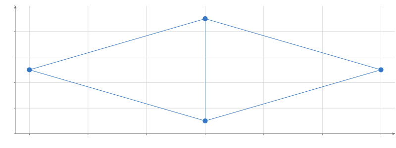
Static preview; loading the interactive plot
import hmplot as hm

data = {"source": ["a", "a", "b", "c", "a"], "target": ["b", "c", "d", "d", "d"]}
with hm.Plot(data=data, height=300) as plot:
    with hm.GraphData(source="source", target="target"):
        with hm.DAG():
            with hm.Edges():
                hm.Routes()
            with hm.Nodes():
                hm.Points(position="position")
plot
Usage
DAG consumes GraphData and uses d3-dag’s Sugiyama layout to place an acyclic directed graph. It exposes node positions and bounds, edge endpoints, and complete routed paths. Routes draws the paths; ordinary edge marks can use start and end. The layout runs when input changes.