HMPlot

Density

A kernel density estimate of one column (a smooth histogram), or of two on a grid (a density heatmap).
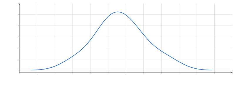
Line chart of density against value. x from -2 to 10, y from -0.01 to 0.3. 256 rows.

Static preview; loading the interactive plot

<script>
  import { Plot, Density, Line } from "hmplot";
  const data = { value: [1.2, 2.5, 2.9, 3.1, 3.4, 3.8, 4.2, 4.4, 5.1, 6.3] };
</script>

<Plot {data} height={300} axes2d>
  <Density x="value">
    <Line x="x" y="density" />
  </Density>
</Plot>

Options

namestring
Names the transform, so a Facet's getTransform(name) reaches its copy in every cell.
xcolumn
The column whose density to estimate; the output's x column holds the points it is evaluated at.
ycolumn
A second column, for a 2D density: the output is a grid of x and y that a Heatmap draws.
bycolumn | column[]
Estimate one density per group of these columns, on the same points; the output keeps these columns.
weightcolumn
Nonnegative weights for the rows.
resolutionnumber | [number, number] | expression
How many points to evaluate: a number, or [nx, ny] in 2D. Default: 256 in 1D, [128, 128] in 2D.
bandwidth"auto" | number | [number, number] | expression
The kernel's width: "auto" uses Scott's rule; a number ([bx, by] in 2D) or an expression such as `multiply(std(col.x), 0.3)` sets it. Default: "auto". In data units.
bounds{x, y}
The range to evaluate over, as {x: [min, max], y: [min, max]}. Default: the data's extent and three bandwidths on each side. In data units.
normalization"density" | "count"
What the density column holds: "density" integrates to 1 over each group; "count" integrates to its row count (or total weight). Default: "density".
as{x, y, density}
New names for the x, y and density columns.

Usage

Outputs x, optional y, and density. 2D output is a grid table (y then x, cell centres that tile the bounds) that Heatmap draws; grouped by one key it gains a leading dimension of the groups. Default resolution is 256 in 1D or 128×128 in 2D; automatic bandwidth uses Scott scaling. by partitions groups; weight accepts nonnegative weights. normalization chooses density or count.

bandwidth="auto" is Scott’s rule. A number sets it directly, and so does an expression evaluated against this transform’s input, such as multiply(std(col.x), 0.3); resolution accepts one too.

To let the viewer change a setting, read an input in it: bandwidth={input("bandwidth")} (Python bandwidth=hm.input.bandwidth), where bandwidth is a Slider.

Related examples

Density estimation